我們使用的是鸢尾花的數據集
python
import numpy as np
import pandas as pd
from matplotlib import pyplot as plt
import math
# 讀取數據源
df = pd.read_csv('E:/file/iris.data')
df.columns=['sepal_len', 'sepal_wid', 'petal_len', 'petal_wid', 'class']
print(df.head())
# 切分數據和標簽
X = df.iloc[:,0:4].values
y = df.iloc[:,4].values
label_dict = {
1: 'Iris-Setosa',
2: 'Iris-Versicolor',
3: 'Iris-Virgnica'}
feature_dict = {
0: 'sepal length [cm]',
1: 'sepal width [cm]',
2: 'petal length [cm]',
3: 'petal width [cm]'}
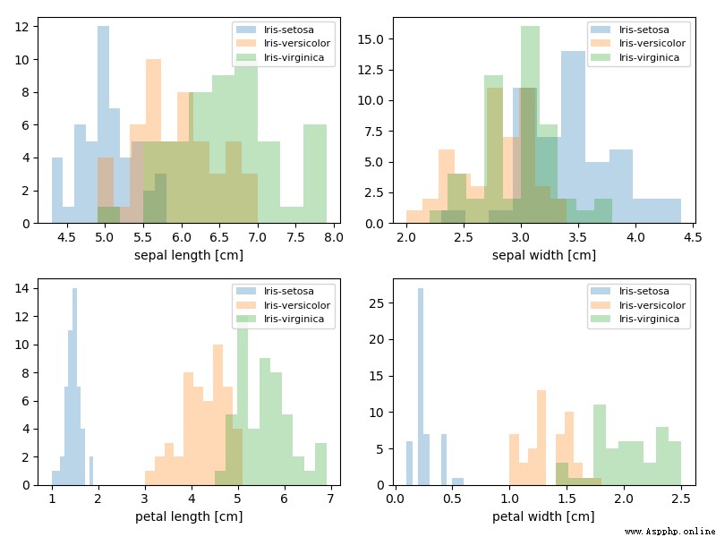
# 畫圖觀測數據集
plt.figure(figsize=(8, 6))
for cnt in range(4):
plt.subplot(2, 2, cnt+1)
for lab in ('Iris-setosa', 'Iris-versicolor', 'Iris-virginica'):
plt.hist(X[y==lab, cnt],
label=lab,
bins=10,
alpha=0.3,)
plt.xlabel(feature_dict[cnt])
plt.legend(loc='upper right', fancybox=True, fontsize=8)
plt.tight_layout()
plt.show()
測試記錄:
 sepal_len sepal_wid petal_len petal_wid class
0 4.9 3.0 1.4 0.2 Iris-setosa
1 4.7 3.2 1.3 0.2 Iris-setosa
2 4.6 3.1 1.5 0.2 Iris-setosa
3 5.0 3.6 1.4 0.2 Iris-setosa
4 5.4 3.9 1.7 0.4 Iris-setosa
代碼:
import numpy as np
import pandas as pd
from matplotlib import pyplot as plt
import math
from sklearn.preprocessing import StandardScaler
# 讀取數據源
df = pd.read_csv('E:/file/iris.data')
df.columns=['sepal_len', 'sepal_wid', 'petal_len', 'petal_wid', 'class']
#print(df.head())
# 切分數據和標簽
X = df.iloc[:,0:4].values
y = df.iloc[:,4].values
# 數據歸一化
X_std = StandardScaler().fit_transform(X)
# 協方差矩陣(對角線元素為1,自身與自身)
cov_mat = np.cov(X_std.T)
# 計算方陣的特征值和特征向量
eig_vals, eig_vecs = np.linalg.eig(cov_mat)
# 生成一個特征值和特征向量的二元組
eig_pairs = [(np.abs(eig_vals[i]), eig_vecs[:,i]) for i in range(len(eig_vals))]
#print(eig_pairs)
#print ('----------')
# 排序
eig_pairs.sort(key=lambda x: x[0], reverse=True)
# 輸出特征值:
print('Eigenvalues in descending order:')
for i in eig_pairs:
print(i[0])
# cumsum求累加值,然後乘100,就是百分比了
tot = sum(eig_vals)
var_exp = [(i / tot)*100 for i in sorted(eig_vals, reverse=True)]
print (var_exp)
cum_var_exp = np.cumsum(var_exp)
cum_var_exp
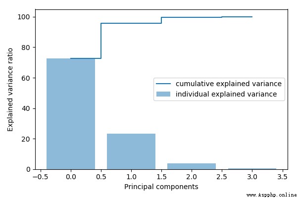
# 畫圖
plt.figure(figsize=(6, 4))
plt.bar(range(4), var_exp, alpha=0.5, align='center',
label='individual explained variance')
plt.step(range(4), cum_var_exp, where='mid',
label='cumulative explained variance')
plt.ylabel('Explained variance ratio')
plt.xlabel('Principal components')
plt.legend(loc='best')
plt.tight_layout()
plt.show()
測試記錄:
Eigenvalues in descending order:
2.9244283691111135
0.9321523302535066
0.1494637348981336
0.02098259276427038
[72.6200333269203, 23.14740685864414, 3.7115155645845284, 0.5210442498510098]
PCA降維的步驟:
代碼:
import numpy as np
import pandas as pd
from matplotlib import pyplot as plt
import math
from sklearn.preprocessing import StandardScaler
# 讀取數據源
df = pd.read_csv('E:/file/iris.data')
df.columns=['sepal_len', 'sepal_wid', 'petal_len', 'petal_wid', 'class']
#print(df.head())
# 切分數據和標簽
X = df.iloc[:,0:4].values
y = df.iloc[:,4].values
# 數據歸一化
X_std = StandardScaler().fit_transform(X)
# 協方差矩陣(對角線元素為1,自身與自身)
cov_mat = np.cov(X_std.T)
# 計算方陣的特征值和特征向量
eig_vals, eig_vecs = np.linalg.eig(cov_mat)
# 生成一個特征值和特征向量的二元組
eig_pairs = [(np.abs(eig_vals[i]), eig_vecs[:,i]) for i in range(len(eig_vals))]
#print(eig_pairs)
#print ('----------')
# 排序
eig_pairs.sort(key=lambda x: x[0], reverse=True)
# 根據特征值生成一個4*2矩陣
matrix_w = np.hstack((eig_pairs[0][1].reshape(4,1),
eig_pairs[1][1].reshape(4,1)))
# 原始矩陣 [15*4] * [4*2] = [15*2] 達到降維的效果
Y = X_std.dot(matrix_w)
# 降維前的效果
plt.figure(figsize=(6, 4))
for lab, col in zip(('Iris-setosa', 'Iris-versicolor', 'Iris-virginica'),
('blue', 'red', 'green')):
plt.scatter(X[y==lab, 0],
X[y==lab, 1],
label=lab,
c=col)
plt.xlabel('sepal_len')
plt.ylabel('sepal_wid')
plt.legend(loc='best')
plt.tight_layout()
#plt.show()
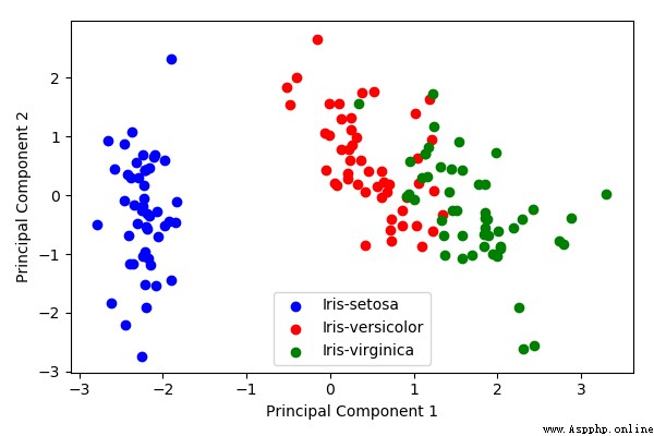
# 降維後的效果
plt.figure(figsize=(6, 4))
for lab, col in zip(('Iris-setosa', 'Iris-versicolor', 'Iris-virginica'),
('blue', 'red', 'green')):
plt.scatter(Y[y==lab, 0],
Y[y==lab, 1],
label=lab,
c=col)
plt.xlabel('Principal Component 1')
plt.ylabel('Principal Component 2')
plt.legend(loc='lower center')
plt.tight_layout()
plt.show()
測試記錄: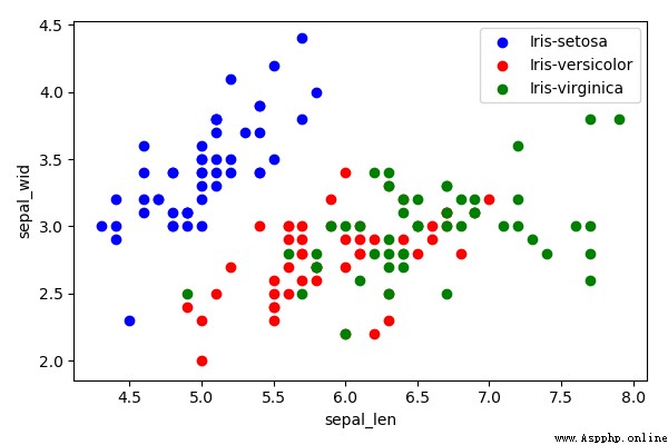
 Super simple to teach you how to clone sound in python (take Juan Fu as an example)
Voice cloning is a popular dee
 I, the post-95 generation, with a monthly salary of 4K to 2w+, from the companys administrative chores to Python engineers, have made up my mind that things can be done
I 95 after , Salary after one