Catalog
Preface
One 、 Introduction
Two 、 The theoretical foundation
Linear separability (linear separability)
hyperplane
Decision boundaries
Support vector (support vector)
Loss function (loss function)
Empirical risk (empirical risk) And structural risk (structural risk)
Nuclear method
Common kernel functions
3、 ... and 、 Algorithm flow
SMO Sequence minimum optimization algorithm
Python sklearn Code implementation :
Python Source code implementation + Handwriting recognition classification :
Focus , Prevent losing , If there is a mistake , Please leave a message , Thank you very much
Refer to the :
Bloggers have participated in dozens of mathematical modeling competitions, large and small ,SVM This model is often seen in excellent papers of various modeling competitions , It is usually used directly SVM There are few algorithms , Now, optimization algorithms are proposed based on this basic theory . however SVM The basic theory of is a very important thought , Look at the whole classification algorithm ,SVM Is the best ready-made classifier . here ‘ Ready-made ’ It means that the classifier can be used directly without modification . Before neural networks appeared ,SVM The optimization model of can be regarded as a prediction and classification artifact , In machine learning SVM It is still one of the most famous algorithms , This blog is dedicated to SVM Every knowledge point of algorithm and principle is explained clearly , I hope you can point out the points you didn't make clear in the comment area .
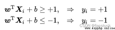
We use SVM Support vector machines are generally used for classification , Get the result of low error rate .SVM It can make good classification decisions for unexpected data points in the training set . First of all, we should look at it from the data level SVM How to make decisions , Here is a diagram of such a series of data sets drawn on a two-dimensional plane coordinate system :
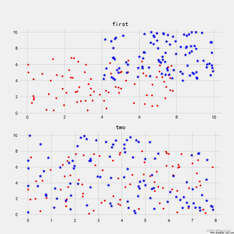
Now we need to consider , Can you draw a straight line to separate circular points from star points . image first Look at the first picture , Dots and stars are very open , It is easy to draw a straight line in the graph to separate the two sets of data . And look at the second picture , Dots and stars almost converge , It's very difficult to distinguish .
If we want to draw a line to distinguish them , There are countless pieces to draw , But it is difficult for us to find the best line with the highest discrimination to distinguish them almost completely . So here we need to understand two basic concepts about data sets :
The data of the first picture is linearly separable , Linear separability visible to the naked eye . The data of the second picture is linear and inseparable . Of course, there is nothing wrong with our straightforward observation , But this is only based on the visualization of two-dimensional plane data , If the feature dimension is higher , for example :
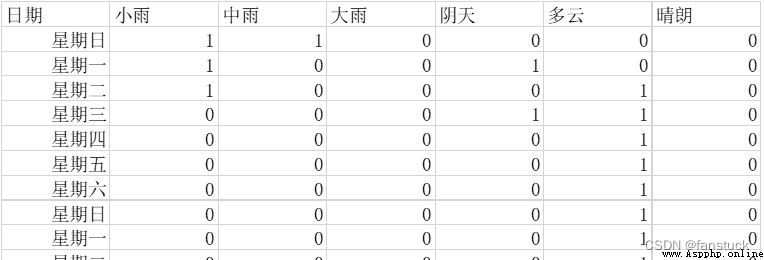
Beyond our visualization technology, how can we judge whether they are separable ?
To judge linear separability, we need to define linear separability :
Given input data and learning objectives in classification problems : ,
, , Each sample of input data contains multiple features and thus forms a feature space (feature space):
 , The learning goal is a binary variable
  Represents a negative class (negative class) Sum positive class (positive class).
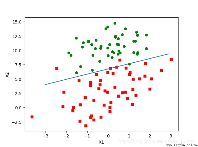
If the feature space where the input data is located exists as the decision boundary (decision boundary) The hyperplane of separates learning objectives into positive and negative classes , And make the distance from the point of any sample to the plane (point to plane distance) Greater than or equal to 1:
decision boundary:
point to plane distance:
The classification problem is said to be linearly separable , Parameters  , They are the normal vector and intercept of the hyperplane .
There must be many friends here who will ask what is the decision boundary and what is the hyperplane , Don't panic and give the definition immediately :
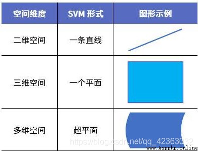
For machine learning , It mostly involves high-dimensional space ( multidimensional ) Data classification of , High dimensional space SVM, That is, hyperplane . The ultimate goal of machine learning is to find the most suitable ( That is, the optimal ) A classification hyperplane (Hyper plane), Thus, using this optimal classification hyperplane, the feature data can be well divided into two categories .
You can understand it by looking at the picture :
In mathematics , hyperplane (Hyperplane) yes n Codimension in a dimensional Euclidean space is equal to 1 The linear subspace of . This is a straight line in the plane 、 Generalization of planes in space . set up F Is the domain ( Consider  ).
).
n Dimensional space  The hyperplane in is determined by the equation :

Defined subset , among  Is a constant that is not all zero .
In the context of linear algebra ,F- Vector space V A hyperplane in is a plane shaped like :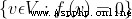
The subspace of , among  Is any nonzero linear mapping .
In projective geometry , Projective space can also be defined  Hyperplane in . In homogeneous coordinates (
 ) The lower hyperplane can be defined by the following equation :
 , among
  Is a constant that is not all zero .
To make a long story short : hyperplane H It's from n Dimension space to n-1 A mapping subspace of dimensional space , It has one n Dimensional vector and a real number definition . set up d yes n Dimensional space R A non-zero vector in ,a Is the set of real Numbers , be R The condition is satisfied in the test dX=a The point of X The set formed is called R A hyperplane in .
SVM It's an optimized classification algorithm , The motivation is to find the best decision boundary , So that there exists between the decision boundary and each group of data margin, And we need to make each side margin Maximize . Then this decision boundary is the boundary between different classes .
To make a long story short : In the statistical classification problem with two classes , The decision boundary or decision surface is a hyperplane , It divides the basic vector space into two sets , A collection . The classifier classifies all points on one side of the decision boundary as belonging to a class , And classify all points on the other side as belonging to another class .
After understanding the hyperplane and decision boundary, we find SVM The core task of is to find a hyperplane as the decision boundary . Then the decision boundary satisfying this condition actually constructs 2 A parallel hyperplane is used as an interval boundary to distinguish the classification of samples :
All samples above the upper interval boundary belong to positive classes , The samples below the lower interval boundary belong to the negative class . The distance between two separation boundaries  Is defined as margin (margin), The positive and negative samples located on the boundary of the interval are support vectors (support vector).
Take our first From the data set of :
No matter how we draw a straight line, there are always lost points that are not correctly classified . When a classification problem does not have linear separability , Using hyperplane as decision boundary will bring classification loss , That is, some support vectors are no longer on the boundary of the interval , Instead, it entered the interior of the interval boundary , Or fall on the wrong side of the decision boundary .
The loss function can quantify the classification loss , Its mathematical form is 0-1 Loss function :

0-1 The loss function is a discontinuous piecewise function , It is not conducive to solving its minimization problem , Therefore, its proxy loss can be constructed in the application (surrogate loss). The proxy loss is consistent with the original loss function (consistency) Loss function of , The model parameter obtained by minimizing the agent loss is also the solution of minimizing the original loss function . That is to say, we need the loss function to calculate the minimum decision boundary . Here is the binary classification (binary classification) in 0-1 Proxy loss of loss function :
name expression Hinge loss function (hinge loss function) Cross entropy loss function (cross-entropy loss function)
 Exponential loss function (exponential loss function)
SVM The hinge loss function is used :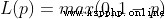 .
.
According to statistical learning theory , The classifier will have risks when it is learned and applied to new data , The types of risks can be divided into empirical risks and structural risks .
empirical risk: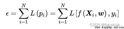
structural risk: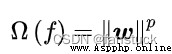
In style  Represents a classifier , Empirical risk is defined by the loss function , Describes the accuracy of the classification results given by the classifier ; Structural risk is defined by the norm of the classifier parameter matrix , Describes the complexity and stability of the classifier itself , Complex classifiers are prone to over fitting , So it's unstable . If a classifier minimizes empirical risk and structural risk A linear combination To determine its model parameters :

Then the solution of the classifier is a regularization problem , constant  It's the regularization coefficient . When
  =2 when , This formula is called
  Regularize or Tikhonov Regularization (Tikhonov regularization).SVM Structural risks
  Express , Hard boundary under linear separable problem SVM The experience risk can be attributed to 0, Therefore, it is a classifier that completely minimizes structural risk ; In the indivisible problem of online , Soft boundary SVM The risk of experience cannot be attributed 0, So it is a Regularization classifier , Minimize the linear combination of structural risk and empirical risk .
Some linear inseparable problems may be nonlinear separable , That is, there is a hyperplane in the feature space to separate positive classes from negative classes . Nonlinear separable problems can be mapped from the original feature space to a higher dimensional space by using nonlinear functions ( Hilbert space (Hilbert space) ) Thus, it is transformed into a linear separable problem , At this time, the hyperplane as the decision boundary is expressed as follows :
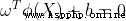
In style  For mapping function . Because the mapping function has a complex form , It is difficult to calculate its inner product , Therefore, the nuclear method can be used (kernel method), That is, define the inner product of the mapping function as a kernel function :
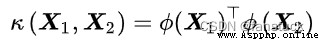
To avoid the explicit calculation of inner product .
 Radial basis function kernel (RBF kernel)
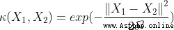 Laplace core (Laplacian kernel)
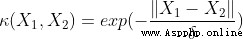 Sigmoid nucleus (Sigmoid kernel)
When the order of polynomial kernel is 1 when , It is called a linear kernel , The corresponding nonlinear classifier degenerates into a linear classifier .RBF Nuclei are also called Gaussian nuclei (Gaussian kernel), Its corresponding mapping function maps the sample space to infinite dimensional space .
After understanding the above algorithm principle , We are right SVM The algorithm has a roughly clear understanding , that SVM How to excavate the hyperplane with the least loss ?
SVM The numerical method of quadratic convex optimization problem can be used to solve , For example, interior point method (Interior Point Method, IPM) And sequence minimum optimization algorithm (Sequential Minimal Optimization, SMO), Random gradient descent can also be used when there are sufficient learning samples .
Here we use SMO Sequence minimum optimization algorithm calculation :
SMO It is a coordinate descent method (coordinate descent) Solve iteratively SVM The dual problem of , Its design is to select two variables in Lagrange multiplier in each iteration step And fix other parameters , The original optimization problem is simplified to one-dimensional sub feasible region , At this time, the constraint has the following equivalent form :
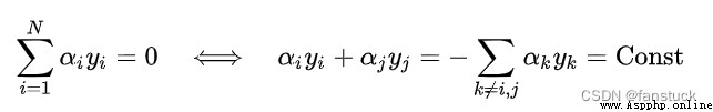
Bring the right side of the above formula into SVM And eliminate the You can get only about  Quadratic programming problem , The optimization problem has a closed form solution and can be calculated quickly . On this basis ,SMO There is the following calculation framework :
Can prove that , In quadratic convex optimization problems ,SMO Each iteration of is strictly optimized SVM The dual problem of , And the iteration will converge to the global maximum after finite steps .SMO The iteration speed of the algorithm and the selected multiplier pair KKT The degree of deviation of conditions , therefore SMO Lagrange multipliers are usually selected by heuristic methods .
For the convenience of showing the effect , We still use it first The data set of :
sklearn.svm.SVC The grammar format is :
class sklearn.svm.SVC( *,
C=1.0,
kernel='rbf',
degree=3,
gamma='scale',
coef0=0.0,
shrinking=True,
probability=False,
tol=0.001,
cache_size=200,
class_weight=None,
verbose=False,
max_iter=- 1,
decision_function_shape='ovr',
break_ties=False,
random_state=None)
The implementation is based on libsvm, More details can be found on the official website :sklearn.svm.SVC.
# The import module
import numpy as np
import matplotlib.pyplot as plt
from sklearn import svm, datasets
# Iris data
iris = datasets.load_iris()
X = iris.data[:, :2] # For the convenience of drawing, only 2 Features
y = iris.target
# Test samples ( Draw the classification area )
xlist1 = np.linspace(X[:, 0].min(), X[:, 0].max(), 200)
xlist2 = np.linspace(X[:, 1].min(), X[:, 1].max(), 200)
XGrid1, XGrid2 = np.meshgrid(xlist1, xlist2)
# nonlinear SVM:RBF nucleus , The super parameter is 0.5, The regularization coefficient is 1,SMO Iterative accuracy 1e-5, Memory footprint 1000MB
svc = svm.SVC(kernel='rbf', C=1, gamma=0.5, tol=1e-5, cache_size=1000).fit(X, y)
# Predict and plot the results
Z = svc.predict(np.vstack([XGrid1.ravel(), XGrid2.ravel()]).T)
Z = Z.reshape(XGrid1.shape)
plt.contourf(XGrid1, XGrid2, Z, cmap=plt.cm.hsv)
plt.contour(XGrid1, XGrid2, Z, colors=('k',))
plt.scatter(X[:, 0], X[:, 1], c=y, edgecolors='k', linewidth=1.5, cmap=plt.cm.hsv)
plt.show() 
from numpy import *
def selectJrand(i, m): # Select an integer randomly in a certain range
# i For the first time alhpa The table below ,m It's all alpha Number of
j = i # we want to select any J not equal to i
while (j == i):
j = int(random.uniform(0, m))
return j
def clipAlpha(aj, H, L): # Adjust the value when it is too large
# aj yes H Is the lower limit , yes L Upper limit
if aj > H:
aj = H
if L > aj:
aj = L
return aj
def kernelTrans(X, A, kTup): # calc the kernel or transform data to a higher dimensional space
# X Is the data ,A yes
m, n = shape(X)
K = mat(zeros((m, 1)))
# And here for simplicity , We only have two built-in kernel functions , But the principle is the same , If necessary, just write other types
# Linear kernel function :k(x,x_i)=x*x_i, It does not need to pass in parameters .
if kTup[0] == 'lin':
K = X * A.T # linear kernel, Linear kernel function
elif kTup[0] == 'rbf': # Gaussian kernel , The parameters passed in as detla
for j in range(m):
deltaRow = X[j, :] - A
K[j] = deltaRow * deltaRow.T # 2 norm
K = exp(K / (-1 * kTup[1] ** 2)) # divide in NumPy is element-wise not matrix like Matlab
# numpy in ,/ Indicates that the matrix elements are calculated instead of the inverse (MATLAB)
else:
raise NameError('Houston We Have a Problem -- \
That Kernel is not recognized')
return K
# Define a class to SMO Algorithm
class optStruct:
def __init__(self, dataMatIn, classLabels, C, toler, kTup): # Initialize the structure with the parameters
# kTup Store kernel information , It's a tuple , The first element of a tuple is a string that describes the type of kernel function , The other two elements are parameters that the kernel function may need
self.X = dataMatIn
self.labelMat = classLabels
self.C = C
self.tol = toler
self.m = shape(dataMatIn)[0] # m It's the number of samples , It's also a The number of
self.alphas = mat(zeros((self.m, 1))) # initialization a Sequence , Set to 0
self.b = 0
# The first column gives eCache Valid flag bit , And the second is practical E value
self.eCache = mat(zeros((self.m, 2))) # first column is valid flag
# If the first one is 1, Explain the current Ek It works
self.K = mat(zeros((self.m, self.m))) # Data calculated with kernel function , Is the inner product matrix , It is convenient to call the inner product result directly
for i in range(self.m):
self.K[:, i] = kernelTrans(self.X, self.X[i, :], kTup)
def calcEk(oS, k): # Computation first k A sample of Ek
fXk = float(multiply(oS.alphas, oS.labelMat).T * oS.K[:, k] + oS.b)
Ek = fXk - float(oS.labelMat[k])
return Ek
def selectJ(i, oS, Ei): # this is the second choice -heurstic, and calcs Ej
# Selected a_1 Then choose a_2
# choice a_2
maxK = -1;
maxDeltaE = 0;
Ej = 0 # choice |E1-E2| maximal E2 And back to E2 and j
# First the E1 Put into , In order to facilitate the later unification
oS.eCache[i] = [1, Ei] # set valid #choose the alpha that gives the maximum delta E
'''
numpy Function returns the directory of non-zero elements .
The return value is a tuple , The two values are two dimensions , Contains the directory value of non-zero elements in the corresponding dimension .
Can pass a[nonzero(a)] To get all non-zero values .
.A It means :getArray(), That is to convert a matrix into an array
'''
# Which samples are obtained Ek It works ,ValidEcacheList There are all valid sample lines Index
validEcacheList = nonzero(oS.eCache[:, 0].A)[0]
# For every effective Ecache Compare them all
if (len(validEcacheList)) > 1:
for k in validEcacheList: # loop through valid Ecache values and find the one that maximizes delta E
if k == i: continue # don't calc for i, waste of time
# If you choose and a1 Same , Just go ahead , because a1 and a2 Different samples must be selected
Ek = calcEk(oS, k)
deltaE = abs(Ei - Ek)
if (deltaE > maxDeltaE):
maxK = k;
maxDeltaE = deltaE;
Ej = Ek
return maxK, Ej
else: # in this case (first time around) we don't have any valid eCache values
j = selectJrand(i, oS.m)
Ej = calcEk(oS, j)
return j, Ej
def updateEk(oS, k): # after any alpha has changed update the new value in the cache
Ek = calcEk(oS, k)
oS.eCache[k] = [1, Ek]
# Calculation Ek And saved in class oS in
# Internal circulation to find the right a_2
def innerL(i, oS):
Ei = calcEk(oS, i) # Why recalculate here ? because a_1 Just updated , Different from the storage
if ((oS.labelMat[i] * Ei < -oS.tol) and (oS.alphas[i] < oS.C)) or (
(oS.labelMat[i] * Ei > oS.tol) and (oS.alphas[i] > 0)):
# If a1 Choose the right words , If it is not appropriate, it will end directly
# The rest of the logic is the same , It's just not using x_ix_j, Instead, use kernel functions
j, Ej = selectJ(i, oS, Ei) # this has been changed from selectJrand
alphaIold = oS.alphas[i].copy();
alphaJold = oS.alphas[j].copy();
if (oS.labelMat[i] != oS.labelMat[j]):
L = max(0, oS.alphas[j] - oS.alphas[i])
H = min(oS.C, oS.C + oS.alphas[j] - oS.alphas[i])
else:
L = max(0, oS.alphas[j] + oS.alphas[i] - oS.C)
H = min(oS.C, oS.alphas[j] + oS.alphas[i])
if L == H: print("L==H"); return 0
eta = 2.0 * oS.K[i, j] - oS.K[i, i] - oS.K[j, j] # changed for kernel
if eta >= 0: print("eta>=0"); return 0
oS.alphas[j] -= oS.labelMat[j] * (Ei - Ej) / eta
oS.alphas[j] = clipAlpha(oS.alphas[j], H, L)
updateEk(oS, j) # added this for the Ecache
if (abs(oS.alphas[j] - alphaJold) < 0.00001): print("j not moving enough"); return 0
oS.alphas[i] += oS.labelMat[j] * oS.labelMat[i] * (alphaJold - oS.alphas[j]) # update i by the same amount as j
updateEk(oS, i) # added this for the Ecache #the update is in the oppostie direction
b1 = oS.b - Ei - oS.labelMat[i] * (oS.alphas[i] - alphaIold) * oS.K[i, i] - oS.labelMat[j] * (
oS.alphas[j] - alphaJold) * oS.K[i, j]
b2 = oS.b - Ej - oS.labelMat[i] * (oS.alphas[i] - alphaIold) * oS.K[i, j] - oS.labelMat[j] * (
oS.alphas[j] - alphaJold) * oS.K[j, j]
if (0 < oS.alphas[i]) and (oS.C > oS.alphas[i]):
oS.b = b1
elif (0 < oS.alphas[j]) and (oS.C > oS.alphas[j]):
oS.b = b2
else:
oS.b = (b1 + b2) / 2.0
return 1
else:
return 0
def smoP(dataMatIn, classLabels, C, toler, maxIter, kTup=('lin', 0)): # The default kernel function is linear , Parameter is 0( That is itself )
# This kTup I don't care , After use
oS = optStruct(mat(dataMatIn), mat(classLabels).transpose(), C, toler, kTup) # Initialize this structure
iter = 0
# entireSet It's a control switch , A loop traverses all sample points , The second time, only traverse the non boundary points
entireSet = True;
alphaPairsChanged = 0
while (iter < maxIter) and ((alphaPairsChanged > 0) or (entireSet)):
alphaPairsChanged: int = 0
if entireSet: # go over all
for i in range(oS.m):
alphaPairsChanged += innerL(i, oS)
print("fullSet, iter: %d i:%d, pairs changed %d" % (iter, i, alphaPairsChanged))
iter += 1
else: # go over non-bound (railed) alphas
# The greater than 0 And less than C Of a_i Pick out , These are non boundary points , Traverse only from these points
nonBoundIs = nonzero((oS.alphas.A > 0) * (oS.alphas.A < C))[0]
for i in nonBoundIs:
alphaPairsChanged += innerL(i, oS)
print("non-bound, iter: %d i:%d, pairs changed %d" % (iter, i, alphaPairsChanged))
iter += 1
# If the first time is for all points , Then the second time is only for non boundary points
# If there is no , On the whole sample
'''
First, select the sample that can make the function value drop enough on the non boundary set as the second variable ,
If there is no , Then select the second variable on the whole sample set ,
If the entire sample set still does not exist , Then re select the first variable .
'''
if entireSet: # After traversing once, it is changed to non boundary traversal
entireSet = False
elif (alphaPairsChanged == 0): # If alpha No updates , Compute the full sample traversal
entireSet = True
print("iteration number: %d" % iter)
return oS.b, oS.alphas
# utilize SVM To classify , Return the function interval , Greater than 0 Belong to 1 class , Less than 0 Belong to 2 class .
def calcWs(alphas, dataArr, classLabels):
X = mat(dataArr);
labelMat = mat(classLabels).transpose()
m, n = shape(X)
w = zeros((n, 1))
for i in range(m):
w += multiply(alphas[i] * labelMat[i], X[i, :].T)
return w
# Convert the image to a vector
def img2vector(filename):
# Altogether 1024 Features
returnVect = zeros((1, 1024))
fr = open(filename)
for i in range(32):
lineStr = fr.readline()
for j in range(32):
returnVect[0, 32 * i + j] = int(lineStr[j])
return returnVect
def loadImages(dirName):
from os import listdir
hwLabels = []
# utilize listdir Read file name , there label Written in the file name
trainingFileList = listdir(dirName) # load the training set
m = len(trainingFileList)
trainingMat = zeros((m, 1024))
for i in range(m):
fileNameStr = trainingFileList[i]
fileStr = fileNameStr.split('.')[0] # take off .txt
classNumStr = int(fileStr.split('_')[0])
if classNumStr == 9:
hwLabels.append(-1)
else:
hwLabels.append(1)
trainingMat[i, :] = img2vector('%s/%s' % (dirName, fileNameStr))
return trainingMat, hwLabels
# Handwriting recognition problem
def testDigits(kTup=('rbf', 10)):
dataArr, labelArr = loadImages('trainingDigits')
b, alphas = smoP(dataArr, labelArr, 200, 0.0001, 10000, kTup)
datMat = mat(dataArr);
labelMat = mat(labelArr).transpose()
svInd = nonzero(alphas.A > 0)[0]
sVs = datMat[svInd]
labelSV = labelMat[svInd];
print("there are %d Support Vectors" % shape(sVs)[0])
m, n = shape(datMat)
errorCount = 0
for i in range(m):
kernelEval = kernelTrans(sVs, datMat[i, :], kTup)
predict = kernelEval.T * multiply(labelSV, alphas[svInd]) + b
if sign(predict) != sign(labelArr[i]): errorCount += 1
print("the training error rate is: %f" % (float(errorCount) / m))
dataArr, labelArr = loadImages('testDigits')
errorCount = 0
datMat = mat(dataArr);
labelMat = mat(labelArr).transpose()
m, n = shape(datMat)
for i in range(m):
kernelEval = kernelTrans(sVs, datMat[i, :], kTup)
predict = kernelEval.T * multiply(labelSV, alphas[svInd]) + b
if sign(predict) != sign(labelArr[i]): errorCount += 1
print("the test error rate is: %f" % (float(errorCount) / m))
testDigits(kTup=('rbf', 20))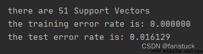
That's what this issue is all about . I am a fanstuck , If you have any questions, please leave a message for discussion , See you next time .
SVM Popular explanation
SVM Baidu Encyclopedia
Loss function Baidu Encyclopedia
Hyperplane Baidu Encyclopedia