來源:B座17樓
由下面代碼生成 
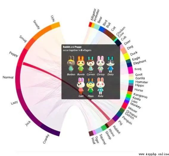
from chord import Chord
matrix = [
[0, 5, 6, 4, 7, 4],
[5, 0, 5, 4, 6, 5],
[6, 5, 0, 4, 5, 5],
[4, 4, 4, 0, 5, 5],
[7, 6, 5, 5, 0, 4],
[4, 5, 5, 5, 4, 0],
]
names = ["Action", "Adventure", "Comedy", "Drama", "Fantasy", "Thriller"]
# 保存
Chord(matrix, names).to_html("chord-diagram.html")
圖形表現力強悍!
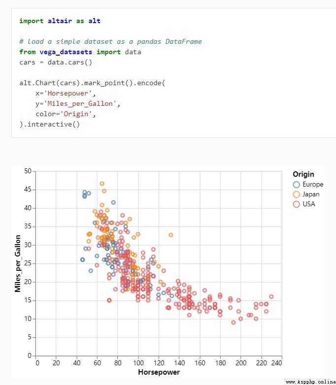
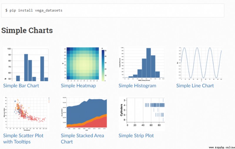
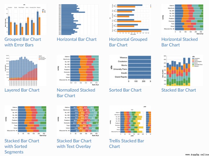
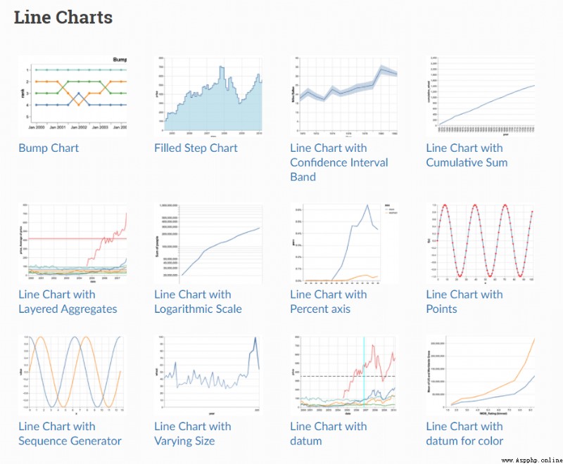
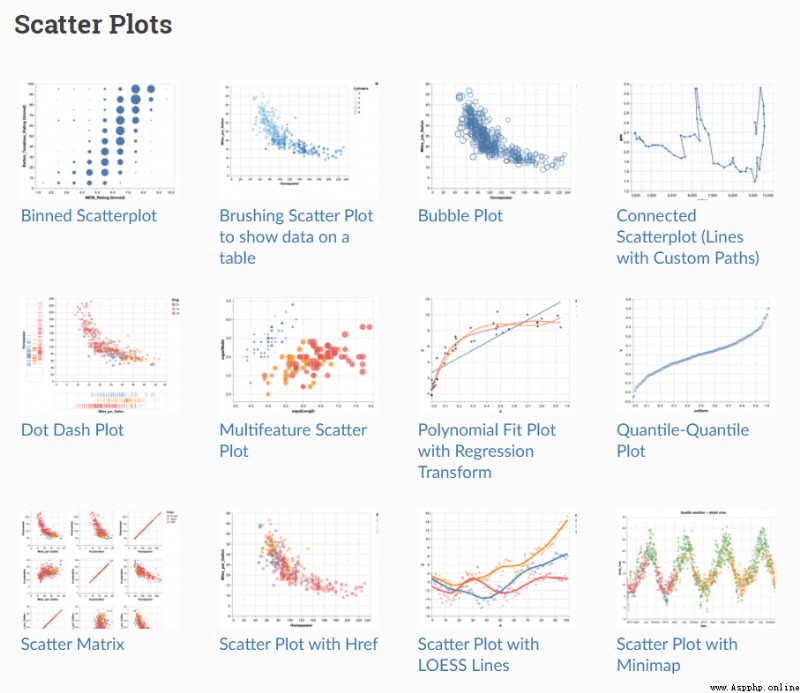
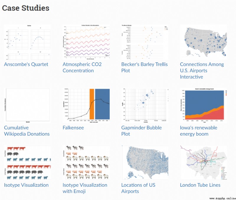
Altair概述
Altair是一個用於Python的聲明式統計可視化庫,基於Vega和Vega-Lite。
Altair提供了一個強大而簡潔的可視化語法,使你能夠快速建立一個廣泛的統計可視化。下面是一個使用Altair API的例子,通過一個交互式散點圖快速實現數據集的可視化。
Github:
https://altair-viz.github.io/getting_started/overview.html
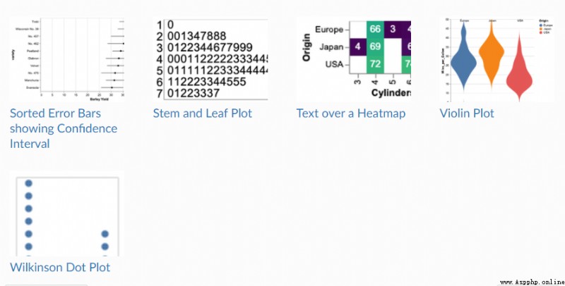
表現強悍
圖形表現力強悍!
import matplotlib.pyplot as plt
# 創建數據
size_of_groups = [12, 11, 3, 30]
# 生成餅圖
plt.pie(size_of_groups)
# 在中心添加一個圓, 生成環形圖
my_circle = plt.Circle((0, 0), 0.7, color='white')
p = plt.gcf()
p.gca().add_artist(my_circle)
plt.show()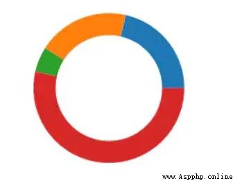
image.png
import matplotlib.pyplot as plt
from matplotlib_venn import venn2
# 創建圖表
venn2(subsets=(10, 5, 2), set_labels=('Group A', 'Group B'))
# 顯示
plt.show()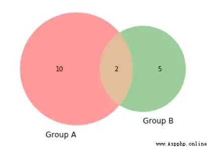
image.png
import circlify
import matplotlib.pyplot as plt
# 創建畫布, 包含一個子圖
fig, ax = plt.subplots(figsize=(14, 14))
# 標題
ax.set_title('Repartition of the world population')
# 移除坐標軸
ax.axis('off')
# 人口數據
data = [{'id': 'World', 'datum': 6964195249, 'children': [
{'id': "North America", 'datum': 450448697,
'children': [
{'id': "United States", 'datum': 308865000},
{'id': "Mexico", 'datum': 107550697},
{'id': "Canada", 'datum': 34033000}
]},
{'id': "South America", 'datum': 278095425,
'children': [
{'id': "Brazil", 'datum': 192612000},
{'id': "Colombia", 'datum': 45349000},
{'id': "Argentina", 'datum': 40134425}
]},
{'id': "Europe", 'datum': 209246682,
'children': [
{'id': "Germany", 'datum': 81757600},
{'id': "France", 'datum': 65447374},
{'id': "United Kingdom", 'datum': 62041708}
]},
{'id': "Africa", 'datum': 311929000,
'children': [
{'id': "Nigeria", 'datum': 154729000},
{'id': "Ethiopia", 'datum': 79221000},
{'id': "Egypt", 'datum': 77979000}
]},
{'id': "Asia", 'datum': 2745929500,
'children': [
{'id': "China", 'datum': 1336335000},
{'id': "India", 'datum': 1178225000},
{'id': "Indonesia", 'datum': 231369500}
]}
]}]
# 使用circlify()計算, 獲取圓的大小, 位置
circles = circlify.circlify(
data,
show_enclosure=False,
target_enclosure=circlify.Circle(x=0, y=0, r=1)
)
lim = max(
max(
abs(circle.x) + circle.r,
abs(circle.y) + circle.r,
)
for circle in circles
)
plt.xlim(-lim, lim)
plt.ylim(-lim, lim)
for circle in circles:
if circle.level != 2:
continue
x, y, r = circle
ax.add_patch(plt.Circle((x, y), r, alpha=0.5, linewidth=2, color="lightblue"))
for circle in circles:
if circle.level != 3:
continue
x, y, r = circle
label = circle.ex["id"]
ax.add_patch(plt.Circle((x, y), r, alpha=0.5, linewidth=2, color="#69b3a2"))
plt.annotate(label, (x, y), ha='center', color="white")
for circle in circles:
if circle.level != 2:
continue
x, y, r = circle
label = circle.ex["id"]
plt.annotate(label, (x, y), va='center', ha='center', bbox=dict(facecolor='white', edgecolor='black', boxstyle='round', pad=.5))
plt.show()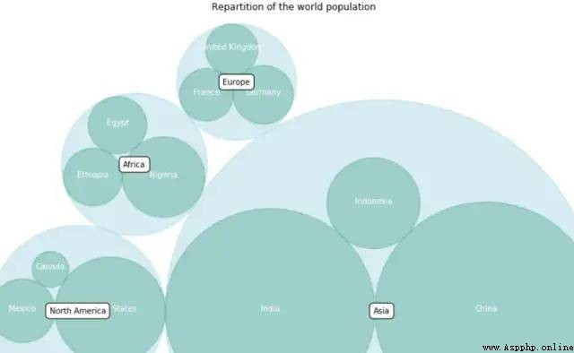
image.png
import folium
import pandas as pd
# 創建地圖對象
m = folium.Map(location=[20,0], tiles="OpenStreetMap", zoom_start=2)
# 坐標點數據
data = pd.DataFrame({
'lon': [-58, 2, 145, 30.32, -4.03, -73.57, 36.82, -38.5],
'lat': [-34, 49, -38, 59.93, 5.33, 45.52, -1.29, -12.97],
'name': ['Buenos Aires', 'Paris', 'melbourne', 'St Petersbourg', 'Abidjan', 'Montreal', 'Nairobi', 'Salvador'],
'value': [10, 12, 40, 70, 23, 43, 100, 43]
}, dtype=str)
# 添加氣泡
for i in range(0, len(data)):
folium.Circle(
location=[data.iloc[i]['lat'], data.iloc[i]['lon']],
popup=data.iloc[i]['name'],
radius=float(data.iloc[i]['value'])*20000,
color='crimson',
fill=True,
fill_color='crimson'
).add_to(m)
# 保存
m.save('bubble-map.html')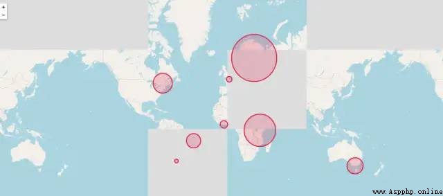
image.png
import altair as alt
from vega_datasets import data
boroughs = alt.topo_feature(data.londonBoroughs.url, 'boroughs')
tubelines = alt.topo_feature(data.londonTubeLines.url, 'line')
centroids = data.londonCentroids.url
background = alt.Chart(boroughs).mark_geoshape(
stroke='white',
strokeWidth=2
).encode(
color=alt.value('#eee'),
).properties(
width=700,
height=500
)
labels = alt.Chart(centroids).mark_text().encode(
longitude='cx:Q',
latitude='cy:Q',
text='bLabel:N',
size=alt.value(8),
opacity=alt.value(0.6)
).transform_calculate(
"bLabel", "indexof (datum.name,' ') > 0 ? substring(datum.name,0,indexof(datum.name, ' ')) : datum.name"
)
line_scale = alt.Scale(domain=["Bakerloo", "Central", "Circle", "District", "DLR",
"Hammersmith & City", "Jubilee", "Metropolitan", "Northern",
"Piccadilly", "Victoria", "Waterloo & City"],
range=["rgb(137,78,36)", "rgb(220,36,30)", "rgb(255,206,0)",
"rgb(1,114,41)", "rgb(0,175,173)", "rgb(215,153,175)",
"rgb(106,114,120)", "rgb(114,17,84)", "rgb(0,0,0)",
"rgb(0,24,168)", "rgb(0,160,226)", "rgb(106,187,170)"])
lines = alt.Chart(tubelines).mark_geoshape(
filled=False,
strokeWidth=2
).encode(
alt.Color(
'id:N',
legend=alt.Legend(
title=None,
orient='bottom-right',
offset=0
),
scale=line_scale
)
)
background + labels + lines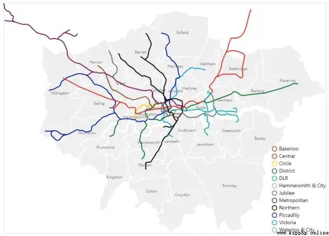
image.png
import altair as alt
from vega_datasets import data
source = data.disasters.url
alt.Chart(source).mark_circle(
opacity=0.8,
stroke='black',
strokeWidth=1
).encode(
alt.X('Year:O', axis=alt.Axis(labelAngle=0)),
alt.Y('Entity:N'),
alt.Size('Deaths:Q',
scale=alt.Scale(range=[0, 4000]),
legend=alt.Legend(title='Annual Global Deaths')
),
alt.Color('Entity:N', legend=None)
).properties(
width=450,
height=320
).transform_filter(
alt.datum.Entity != 'All natural disasters'
)
image.png
import altair as alt
import pandas as pd
source = pd.DataFrame([
{'country': 'Great Britain', 'animal': 'cattle'},
{'country': 'Great Britain', 'animal': 'cattle'},
{'country': 'Great Britain', 'animal': 'cattle'},
{'country': 'Great Britain', 'animal': 'pigs'},
{'country': 'Great Britain', 'animal': 'pigs'},
{'country': 'Great Britain', 'animal': 'sheep'},
{'country': 'Great Britain', 'animal': 'sheep'},
{'country': 'Great Britain', 'animal': 'sheep'},
{'country': 'Great Britain', 'animal': 'sheep'},
{'country': 'Great Britain', 'animal': 'sheep'},
{'country': 'Great Britain', 'animal': 'sheep'},
{'country': 'Great Britain', 'animal': 'sheep'},
{'country': 'Great Britain', 'animal': 'sheep'},
{'country': 'Great Britain', 'animal': 'sheep'},
{'country': 'Great Britain', 'animal': 'sheep'},
{'country': 'United States', 'animal': 'cattle'},
{'country': 'United States', 'animal': 'cattle'},
{'country': 'United States', 'animal': 'cattle'},
{'country': 'United States', 'animal': 'cattle'},
{'country': 'United States', 'animal': 'cattle'},
{'country': 'United States', 'animal': 'cattle'},
{'country': 'United States', 'animal': 'cattle'},
{'country': 'United States', 'animal': 'cattle'},
{'country': 'United States', 'animal': 'cattle'},
{'country': 'United States', 'animal': 'pigs'},
{'country': 'United States', 'animal': 'pigs'},
{'country': 'United States', 'animal': 'pigs'},
{'country': 'United States', 'animal': 'pigs'},
{'country': 'United States', 'animal': 'pigs'},
{'country': 'United States', 'animal': 'pigs'},
{'country': 'United States', 'animal': 'sheep'},
{'country': 'United States', 'animal': 'sheep'},
{'country': 'United States', 'animal': 'sheep'},
{'country': 'United States', 'animal': 'sheep'},
{'country': 'United States', 'animal': 'sheep'},
{'country': 'United States', 'animal': 'sheep'},
{'country': 'United States', 'animal': 'sheep'}
])
domains = ['person', 'cattle', 'pigs', 'sheep']
shape_scale = alt.Scale(
domain=domains,
range=[
'M1.7 -1.7h-0.8c0.3 -0.2 0.6 -0.5 0.6 -0.9c0 -0.6 -0.4 -1 -1 -1c-0.6 0 -1 0.4 -1 1c0 0.4 0.2 0.7 0.6 0.9h-0.8c-0.4 0 -0.7 0.3 -0.7 0.6v1.9c0 0.3 0.3 0.6 0.6 0.6h0.2c0 0 0 0.1 0 0.1v1.9c0 0.3 0.2 0.6 0.3 0.6h1.3c0.2 0 0.3 -0.3 0.3 -0.6v-1.8c0 0 0 -0.1 0 -0.1h0.2c0.3 0 0.6 -0.3 0.6 -0.6v-2c0.2 -0.3 -0.1 -0.6 -0.4 -0.6z',
'M4 -2c0 0 0.9 -0.7 1.1 -0.8c0.1 -0.1 -0.1 0.5 -0.3 0.7c-0.2 0.2 1.1 1.1 1.1 1.2c0 0.2 -0.2 0.8 -0.4 0.7c-0.1 0 -0.8 -0.3 -1.3 -0.2c-0.5 0.1 -1.3 1.6 -1.5 2c-0.3 0.4 -0.6 0.4 -0.6 0.4c0 0.1 0.3 1.7 0.4 1.8c0.1 0.1 -0.4 0.1 -0.5 0c0 0 -0.6 -1.9 -0.6 -1.9c-0.1 0 -0.3 -0.1 -0.3 -0.1c0 0.1 -0.5 1.4 -0.4 1.6c0.1 0.2 0.1 0.3 0.1 0.3c0 0 -0.4 0 -0.4 0c0 0 -0.2 -0.1 -0.1 -0.3c0 -0.2 0.3 -1.7 0.3 -1.7c0 0 -2.8 -0.9 -2.9 -0.8c-0.2 0.1 -0.4 0.6 -0.4 1c0 0.4 0.5 1.9 0.5 1.9l-0.5 0l-0.6 -2l0 -0.6c0 0 -1 0.8 -1 1c0 0.2 -0.2 1.3 -0.2 1.3c0 0 0.3 0.3 0.2 0.3c0 0 -0.5 0 -0.5 0c0 0 -0.2 -0.2 -0.1 -0.4c0 -0.1 0.2 -1.6 0.2 -1.6c0 0 0.5 -0.4 0.5 -0.5c0 -0.1 0 -2.7 -0.2 -2.7c-0.1 0 -0.4 2 -0.4 2c0 0 0 0.2 -0.2 0.5c-0.1 0.4 -0.2 1.1 -0.2 1.1c0 0 -0.2 -0.1 -0.2 -0.2c0 -0.1 -0.1 -0.7 0 -0.7c0.1 -0.1 0.3 -0.8 0.4 -1.4c0 -0.6 0.2 -1.3 0.4 -1.5c0.1 -0.2 0.6 -0.4 0.6 -0.4z',
'M1.2 -2c0 0 0.7 0 1.2 0.5c0.5 0.5 0.4 0.6 0.5 0.6c0.1 0 0.7 0 0.8 0.1c0.1 0 0.2 0.2 0.2 0.2c0 0 -0.6 0.2 -0.6 0.3c0 0.1 0.4 0.9 0.6 0.9c0.1 0 0.6 0 0.6 0.1c0 0.1 0 0.7 -0.1 0.7c-0.1 0 -1.2 0.4 -1.5 0.5c-0.3 0.1 -1.1 0.5 -1.1 0.7c-0.1 0.2 0.4 1.2 0.4 1.2l-0.4 0c0 0 -0.4 -0.8 -0.4 -0.9c0 -0.1 -0.1 -0.3 -0.1 -0.3l-0.2 0l-0.5 1.3l-0.4 0c0 0 -0.1 -0.4 0 -0.6c0.1 -0.1 0.3 -0.6 0.3 -0.7c0 0 -0.8 0 -1.5 -0.1c-0.7 -0.1 -1.2 -0.3 -1.2 -0.2c0 0.1 -0.4 0.6 -0.5 0.6c0 0 0.3 0.9 0.3 0.9l-0.4 0c0 0 -0.4 -0.5 -0.4 -0.6c0 -0.1 -0.2 -0.6 -0.2 -0.5c0 0 -0.4 0.4 -0.6 0.4c-0.2 0.1 -0.4 0.1 -0.4 0.1c0 0 -0.1 0.6 -0.1 0.6l-0.5 0l0 -1c0 0 0.5 -0.4 0.5 -0.5c0 -0.1 -0.7 -1.2 -0.6 -1.4c0.1 -0.1 0.1 -1.1 0.1 -1.1c0 0 -0.2 0.1 -0.2 0.1c0 0 0 0.9 0 1c0 0.1 -0.2 0.3 -0.3 0.3c-0.1 0 0 -0.5 0 -0.9c0 -0.4 0 -0.4 0.2 -0.6c0.2 -0.2 0.6 -0.3 0.8 -0.8c0.3 -0.5 1 -0.6 1 -0.6z',
'M-4.1 -0.5c0.2 0 0.2 0.2 0.5 0.2c0.3 0 0.3 -0.2 0.5 -0.2c0.2 0 0.2 0.2 0.4 0.2c0.2 0 0.2 -0.2 0.5 -0.2c0.2 0 0.2 0.2 0.4 0.2c0.2 0 0.2 -0.2 0.4 -0.2c0.1 0 0.2 0.2 0.4 0.1c0.2 0 0.2 -0.2 0.4 -0.3c0.1 0 0.1 -0.1 0.4 0c0.3 0 0.3 -0.4 0.6 -0.4c0.3 0 0.6 -0.3 0.7 -0.2c0.1 0.1 1.4 1 1.3 1.4c-0.1 0.4 -0.3 0.3 -0.4 0.3c-0.1 0 -0.5 -0.4 -0.7 -0.2c-0.3 0.2 -0.1 0.4 -0.2 0.6c-0.1 0.1 -0.2 0.2 -0.3 0.4c0 0.2 0.1 0.3 0 0.5c-0.1 0.2 -0.3 0.2 -0.3 0.5c0 0.3 -0.2 0.3 -0.3 0.6c-0.1 0.2 0 0.3 -0.1 0.5c-0.1 0.2 -0.1 0.2 -0.2 0.3c-0.1 0.1 0.3 1.1 0.3 1.1l-0.3 0c0 0 -0.3 -0.9 -0.3 -1c0 -0.1 -0.1 -0.2 -0.3 -0.2c-0.2 0 -0.3 0.1 -0.4 0.4c0 0.3 -0.2 0.8 -0.2 0.8l-0.3 0l0.3 -1c0 0 0.1 -0.6 -0.2 -0.5c-0.3 0.1 -0.2 -0.1 -0.4 -0.1c-0.2 -0.1 -0.3 0.1 -0.4 0c-0.2 -0.1 -0.3 0.1 -0.5 0c-0.2 -0.1 -0.1 0 -0.3 0.3c-0.2 0.3 -0.4 0.3 -0.4 0.3l0.2 1.1l-0.3 0l-0.2 -1.1c0 0 -0.4 -0.6 -0.5 -0.4c-0.1 0.3 -0.1 0.4 -0.3 0.4c-0.1 -0.1 -0.2 1.1 -0.2 1.1l-0.3 0l0.2 -1.1c0 0 -0.3 -0.1 -0.3 -0.5c0 -0.3 0.1 -0.5 0.1 -0.7c0.1 -0.2 -0.1 -1 -0.2 -1.1c-0.1 -0.2 -0.2 -0.8 -0.2 -0.8c0 0 -0.1 -0.5 0.4 -0.8z'
]
)
color_scale = alt.Scale(
domain=domains,
range=['rgb(162,160,152)', 'rgb(194,81,64)', 'rgb(93,93,93)', 'rgb(91,131,149)']
)
alt.Chart(source).mark_point(filled=True, opacity=1, size=100).encode(
alt.X('x:O', axis=None),
alt.Y('animal:O', axis=None),
alt.Row('country:N', header=alt.Header(title='')),
alt.Shape('animal:N', legend=None, scale=shape_scale),
alt.Color('animal:N', legend=None, scale=color_scale),
).transform_window(
x='rank()',
groupby=['country', 'animal']
).properties(width=550, height=140)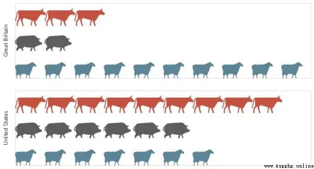
提供豐富的圖形代碼
推薦閱讀 點擊標題可跳轉
Python學習手冊
Pandas學習大禮包
100+Python爬蟲項目
Python數據分析入門手冊
浙江大學內部Python教程
240個Python練習案例附源碼
70個Python經典實用練手項目
整理了30款Python小游戲附源碼
 Official recommendation: there are six ways for pandas to read excel, and the correct answers are written in the source code ~ its too convenient
Hello everyone , This is Wang
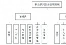 Computer graduation design Python + djang newborn registration service management system (source + + mysql database system + Lw document)
項目介紹Every year, a large number