Recently, some software search questions 、 The function of intelligent correction should be offline .
refund 1024 Step talk , Do you want to make an automatic correction function ? What if one day the child wants to use it !
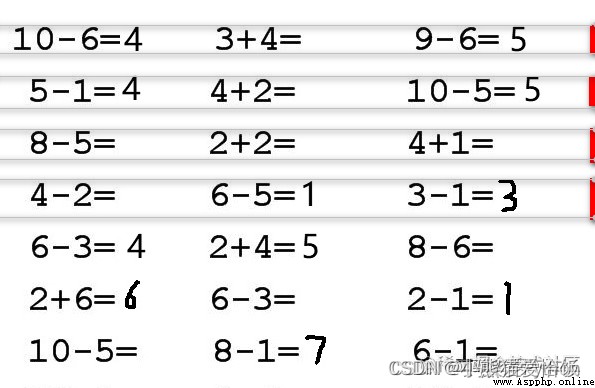
I had a dream last night , I dreamed that I realized this function , As shown in the figure below :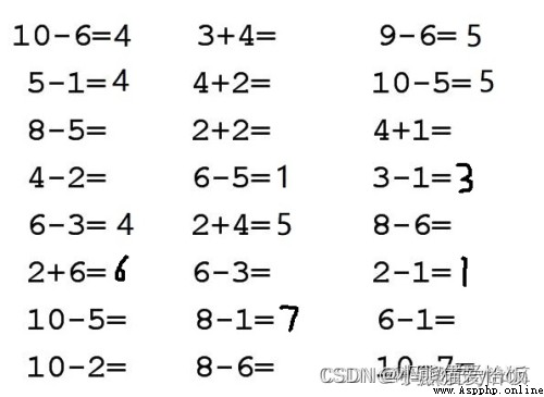 Function introduction : Right , Can make a right sign ; Do wrong , Can cross ; What you didn't do , Can you fill in the answer .
After waking up , I look around , Lie down again , I hope the dream can connect .
The basic idea
Actually , Just finish it at two o'clock , The first is to be able to recognize numbers , The second is to be able to segment numbers .
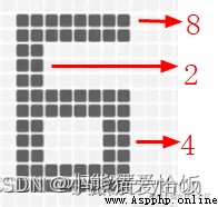
First of all, you have to know 5 yes 5, This is a prerequisite , The second is to find 5、6、7、8 The location of these digital areas .
The former is image recognition , The latter is image cutting .
• For image recognition , The general routine is as follows (CNN Convolutional neural networks ):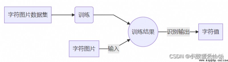 For image cutting , The general routine is as follows ( Transverse and longitudinal projection method ):
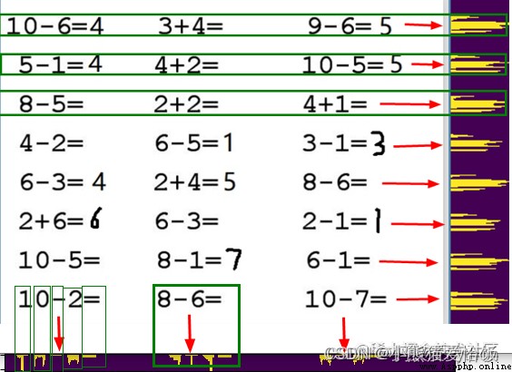 Since the idea can work , Let's start with image recognition . Prepare the data -> Train the data and save the model -> Use the training model to predict the results .
For boyfriend , Find a glib Playboy , Why don't you find a muggy gourd IT male , Train him to be what you want him to be .
We don't need any official mnist Data sets , Because it's official , Is not your , You want to add ±×÷ It doesn't either .
Some common data sets , Although it's powerful , Very convenient , But once you put it in your scene , The effect is not as good as your wish .
Only train your own data , Then you can use it yourself . what's more , We enjoy the process of creation .
hypothesis , We only recognize oral arithmetic , Then the image data we need are as follows :
 Indexes :0 1 2 3 4 5 6 7 8 9 10 11 12 13 14
character :0 1 2 3 4 5 6 7 8 9 = + - × ÷
If you can identify these , It can basically meet the addition, subtraction, multiplication and division of integers .
Okay , Where did the picture come from ?!
Yeah , Where did the picture come from ?
I almost woke up from my dream ,500 Wandu has planned how to spend , Actually, the two-color ball has not been selected yet !
In my dream , An old man told me , Pictures should be generated by yourself . I asked him how to generate , He chuckled , Disappear into the fog ……
Think carefully , It's not hard , We always type , Generating numbers is nothing more than writing words on pictures with code .
The reason why words can show , Mainly because of the support of Fonts .
If you're using a windows System , Then open KaTeX parse error: Undefined control sequence: \Windows at position 3: C:\̲W̲i̲n̲d̲o̲w̲s̲\Fonts This folder , You'll find a lot of Fonts .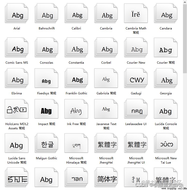 We write code to call these Fonts , Then print it on a picture , Is there data .
And these data are completely under our control , As much as you want , Think less, think less , Think about numbers 、 Letter 、 Chinese characters 、 Symbols are OK , You worked out digital recognition today , Also phase
When you have all the identifications at the same time ! I'm a little excited to think about it !
have a look , This is the difference between working and starting a business . Using other people's data is equivalent to working , You don't have to worry about , But you have what he gives you . Making your own data is quite
Start a business , Although the early stage is hard , You can completely control the rhythm yourself , Add... If necessary , Remove if it's useless .
To build a fonts Folder , Copy some fonts from the font library and put them in , I have a copy here 13 A font file .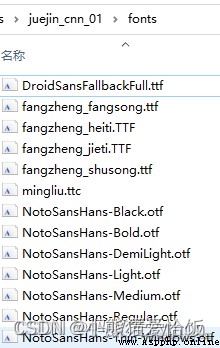 well , The preparations are ready , Must be very tired , Rest rest rest , I'll do it later !
The code is as follows , It can run directly .
python Exchange of learning Q Group :660193417###
from __future__ import print_function
from PIL import Image
from PIL import ImageFont
from PIL import ImageDraw
import os
import shutil
import time
# %% Text to be generated
label_dict = {0: '0', 1: '1', 2: '2', 3: '3', 4: '4', 5: '5', 6: '6', 7: '7', 8: '8', 9: '9', 10: '=', 11: '+', 12: '-', 13: '×', 14: '÷'}
# The folder corresponding to the text , Create a file for each category
for value,char in label_dict.items():
train_images_dir = "dataset"+"/"+str(value)
if os.path.isdir(train_images_dir):
shutil.rmtree(train_images_dir)
os.makedirs(train_images_dir)
# %% Generate pictures
def makeImage(label\_dict, font\_path, width=24, height=24, rotate = 0):
# Take the key value pair from the dictionary
for value,char in label_dict.items():
# Create a picture with a black background , Size is 24*24
img = Image.new("RGB", (width, height), "black")
draw = ImageDraw.Draw(img)
# Load a font , The font size is the width of the picture 90%
font = ImageFont.truetype(font_path, int(width*0.9))
# Gets the width and height of the font
font_width, font_height = draw.textsize(char, font)
# Calculate the font drawn x,y coordinate , The main thing is to draw the text in the center of the icon
x = (width - font_width-font.getoffset(char)[0]) / 2
y = (height - font_height-font.getoffset(char)[1]) / 2
# Drawing pictures , Draw there , Draw what , What color , What font
draw.text((x,y), char, (255, 255, 255), font)
# Set the tilt angle of the picture
img = img.rotate(rotate)
# Named file save , Naming rules :dataset/ Number /img- Number \_r- Choose the angle \_ Time stamp .png
time_value = int(round(time.time() * 1000))
img_path = "dataset/{}/img-{}\_r-{}\_{}.png".format(value,value,rotate,time_value)
img.save(img_path)
# %% The path where the font is stored
font_dir = "./fonts"
for font_name in os.listdir(font_dir):
# Take out every font , Each font generates a batch of pictures
path_font_file = os.path.join(font_dir, font_name)
# The tilt angle is from -10 To 10 degree , Each angle generates a batch of pictures
for k in range(-10, 10, 1):
# Each character generates a picture
makeImage(label_dict, path_font_file, rotate = k)
Fold
The pure code above is less than 30 That's ok , I believe you should be able to understand ! I don't understand. It's not my reader .
The core code is to draw text .
draw.text((x,y), char, (255, 255, 255), font)
Translation is : Use a font in the black background of the picture (x,y) The position is written in white char Symbol .
The core logic is a three-tier loop .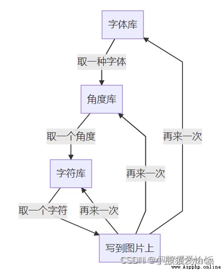 If the code you run is OK , Finally, the following results will be generated :
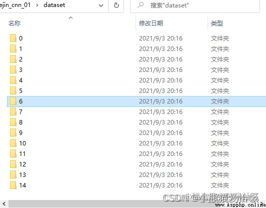
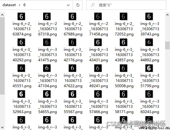 Okay , The data is ready . in total 15 A folder , The corresponding character pictures of various fonts and tilt angles under each folder 3900 individual ( character 15 class × typeface 13 Kind of × angle 20 individual ), The size of the picture is 24×24 Pixels .
With data , We can move on to the next step , The next step is to train and use the data .
2.2.1 To build a model, you first look at the code , The layman feels so profound , An expert laughs secretly .
# %% Import necessary packages
import tensorflow as tf
import numpy as np
from tensorflow.keras import layers
from tensorflow.keras.models import Sequential
import pathlib
import cv2
# %% Build the model
def create\_model():
model = Sequential([
layers.experimental.preprocessing.Rescaling(1./255, input_shape=(24, 24, 1)),
layers.Conv2D(24,3,activation='relu'),
layers.MaxPooling2D((2,2)),
layers.Conv2D(64,3, activation='relu'),
layers.MaxPooling2D((2,2)),
layers.Flatten(),
layers.Dense(128, activation='relu'),
layers.Dense(15)]
)
model.compile(optimizer='adam',
loss=tf.keras.losses.SparseCategoricalCrossentropy(from_logits=True),
metrics=['accuracy'])
return model
The sequence of this model is as follows , The function is to input a picture data , Knead through each layer , Finally predict which category this picture belongs to .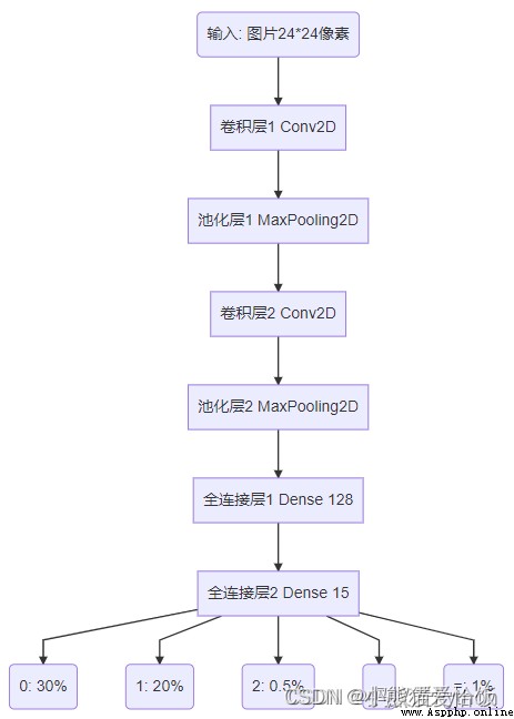 What are these layers for , What's the usage? ? Like clothes , It must be useful , Underwear 、 shirt 、 sweater 、 Cotton padded clothes have their own uses .
Investigators from various functional departments , Collect and sort out specific data in a unit area . What we input is an image , It's made up of pixels , This is it. R e s c a l i
n g ( 1. / 255 , i n p u t s h a p e = ( 24 , 24 , 1 ) ) Rescaling(1./255, input_shape=(24, 24, 1))Rescaling(1./255,input shape=(24,24,1)) in ,
input_shape The input shape is 24*24 Pixels 1 Channels ( Color is RGB 3 Channels ) Image .
 The definition in convolution layer code is Conv2D(24,3), It means to use 3*3 Convolution kernel of pixels , To extract 24 Features .
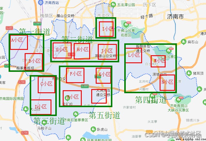
I turn the map to the map , You can understand . Take Shizhong District of Jinan as an example .
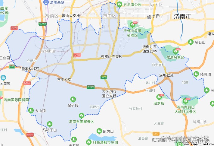 The function of convolution is equivalent to collecting multiple groups of specific information from a certain level unit area of the map . For example, take the community as the unit to extract the number of houses 、 The number of parking spaces 、 Number of schools 、 Population 、 Annual income 、 Education 、 Age and so on 24 Information of dimensions . A cell is equivalent to a convolution kernel .
After the extraction is completed, it is like this .
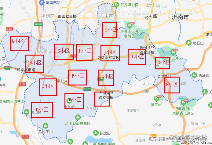 After the first convolution , We got... From downtown N Cell data .
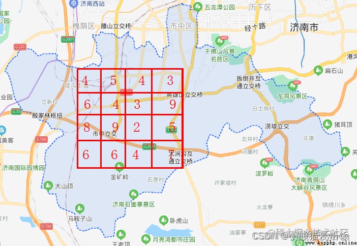
Convolution can be performed many times .
For example, after cell convolution , We can also do it again on the basis of the community , Here is the street .
 By convoluting the community in street units again , We got it from Shizhong District N Data of two streets .
This is the function of convolution .
Through convolution , Just take a big picture , Roll it up in a specific way , What is left behind is a fixed set of purposeful data , So as to facilitate the subsequent selection decision . This is the data of selecting a district , If we choose Jinan , Even Shandong Province , The same is true . This is similar to the selection of civilized cities in real life 、 It is also a truth that the economy is strong .
To put it bluntly, it's rounding .
The computing power of the computer is powerful , Faster than you and me , But not without considering the cost . We certainly want it to be as fast as possible , If one method can save half the time , We are certainly willing to use this method .
This is what the pool layer does . The code definition of pooling is like this M a x P o o l i n g 2 D ( ( 2 , 2 ) )MaxPooling2D((2,2))MaxPooling2D((2,2)), Here is the maximum pool . among (2,2) Is the size of the pool layer , In fact, in the 2*2 In the area , We think this piece can be combined into a unit .
Take another example of a map , Like the following 16 Data in a grid , yes 16 Number of schools in one street .
 In order to further improve the computational efficiency , Calculate less data , We use it 2*2 Pool the pool layer .
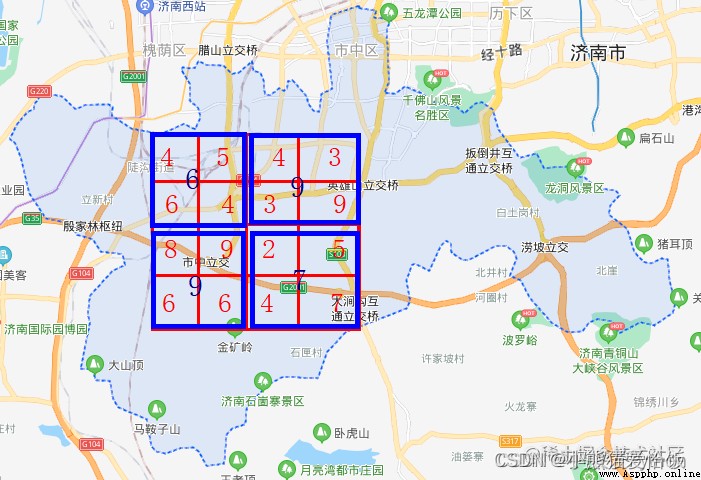 The square of pool is 4 Two streets are combined 1 individual , The number of schools in the new unit is the largest among the members ( Also take the smallest , Take the average number of pools ) The one of . After pooling ,
16 A grid becomes 4 Lattice , This reduces data .
This is the role of the pool layer .
Weak water three thousand , Only take a gourd ladle .
ad locum , It's actually a classifier .
When we build it , The code looks like this D e n s e ( 15 ) Dense(15)Dense(15).
What it does , No matter what's in front of you , How many dimensions , To me, I will forcibly convert it into a fixed channel .
For example, identifying letters a~z, I have a 500 Neurons are involved in judgment , But the final output is 26 Channels (a,b,c,……,y,z).
We have a total of 15 Class characters , So it is 15 Channels . Given an input , Output the probability for each classification .
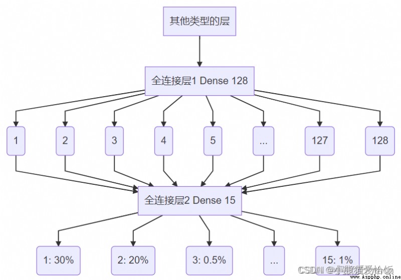 Be careful : It's all two-dimensional input , such as 24×24, But the full connection layer is one-dimensional , So the code uses l a y e r s . F l a t t e n ( )
layers.Flatten()layers.Flatten() Flatten the two-dimensional data into one-dimensional data ([[11,12],[21,22]]->[11,12,21,22]).
For the overall model , call m o d e l . s u m m a r y ( ) model.summary()model.summary() The network structure of the print sequence is as follows :
\_\_\_\_\_\_\_\_\_\_\_\_\_\_\_\_\_\_\_\_\_\_\_\_\_\_\_\_\_\_\_\_\_\_\_\_\_\_\_\_\_\_\_\_\_\_\_\_\_\_\_\_\_\_\_\_\_\_\_\_\_\_\_\_\_
Layer (type) Output Shape Param #
=================================================================
rescaling\_2 (Rescaling) (None, 24, 24, 1) 0
\_\_\_\_\_\_\_\_\_\_\_\_\_\_\_\_\_\_\_\_\_\_\_\_\_\_\_\_\_\_\_\_\_\_\_\_\_\_\_\_\_\_\_\_\_\_\_\_\_\_\_\_\_\_\_\_\_\_\_\_\_\_\_\_\_
conv2d\_4 (Conv2D) (None, 22, 22, 24) 240
\_\_\_\_\_\_\_\_\_\_\_\_\_\_\_\_\_\_\_\_\_\_\_\_\_\_\_\_\_\_\_\_\_\_\_\_\_\_\_\_\_\_\_\_\_\_\_\_\_\_\_\_\_\_\_\_\_\_\_\_\_\_\_\_\_
max\_pooling2d\_4 (MaxPooling2 (None, 11, 11, 24) 0
\_\_\_\_\_\_\_\_\_\_\_\_\_\_\_\_\_\_\_\_\_\_\_\_\_\_\_\_\_\_\_\_\_\_\_\_\_\_\_\_\_\_\_\_\_\_\_\_\_\_\_\_\_\_\_\_\_\_\_\_\_\_\_\_\_
conv2d\_5 (Conv2D) (None, 9, 9, 64) 13888
\_\_\_\_\_\_\_\_\_\_\_\_\_\_\_\_\_\_\_\_\_\_\_\_\_\_\_\_\_\_\_\_\_\_\_\_\_\_\_\_\_\_\_\_\_\_\_\_\_\_\_\_\_\_\_\_\_\_\_\_\_\_\_\_\_
max\_pooling2d\_5 (MaxPooling2 (None, 4, 4, 64) 0
\_\_\_\_\_\_\_\_\_\_\_\_\_\_\_\_\_\_\_\_\_\_\_\_\_\_\_\_\_\_\_\_\_\_\_\_\_\_\_\_\_\_\_\_\_\_\_\_\_\_\_\_\_\_\_\_\_\_\_\_\_\_\_\_\_
flatten\_2 (Flatten) (None, 1024) 0
\_\_\_\_\_\_\_\_\_\_\_\_\_\_\_\_\_\_\_\_\_\_\_\_\_\_\_\_\_\_\_\_\_\_\_\_\_\_\_\_\_\_\_\_\_\_\_\_\_\_\_\_\_\_\_\_\_\_\_\_\_\_\_\_\_
dense\_4 (Dense) (None, 128) 131200
\_\_\_\_\_\_\_\_\_\_\_\_\_\_\_\_\_\_\_\_\_\_\_\_\_\_\_\_\_\_\_\_\_\_\_\_\_\_\_\_\_\_\_\_\_\_\_\_\_\_\_\_\_\_\_\_\_\_\_\_\_\_\_\_\_
dense\_5 (Dense) (None, 15) 1935
=================================================================
Total params: 147,263
Trainable params: 147,263
Non-trainable params: 0
\_\_\_\_\_\_\_\_\_\_\_\_\_\_\_\_\_\_\_\_\_\_\_\_\_\_\_\_\_\_\_\_\_\_\_\_\_\_\_\_\_\_\_\_\_\_\_\_\_\_\_\_\_\_\_\_\_\_\_\_\_\_\_\_\_
We see conv2d_5 (Conv2D) (None, 9, 9, 64) after 2*2 After pooling, it becomes max_pooling2d_5 (MaxPooling2 (None, 4, 4, 64).(None,
4, 4, 64) after F l a t t e n FlattenFlatten After being pulled into one dimension, it becomes (None, 1024), After full connection, it becomes (None, 128) Once again, the full connection becomes (None,
15),15 Is our final classification . We designed all this .
m o d e l . c o m p i l e model.compilemodel.compile Just a few parameters of the configuration model , Just remember this at this stage .
Execution is over .
python Exchange of learning Q Group :660193417####
# Count the number of all pictures in the folder
data_dir = pathlib.Path('dataset')
# Read pictures from folder , Generate data set
train_ds = tf.keras.preprocessing.image_dataset_from_directory(
data_dir, # Which file to get data from
color_mode="grayscale", # The color of the acquired data is grayscale
image_size=(24, 24), # The size of the picture
batch_size=32 # How many pictures are a batch
)
# Classification of data sets , Corresponding dataset How many pictures are classified under the folder
class_names = train_ds.class_names
# Save dataset classification
np.save("class\_name.npy", class_names)
# Data set cache processing
AUTOTUNE = tf.data.experimental.AUTOTUNE
train_ds = train_ds.cache().shuffle(1000).prefetch(buffer_size=AUTOTUNE)
# Creating models
model = create_model()
# Training models ,epochs=10, All data sets are trained 10 All over
model.fit(train_ds,epochs=10)
# Save the weight after training
model.save_weights('checkpoint/char_checkpoint')
After execution, the following information will be output :
Found 3900 files belonging to 15 classes.
Epoch 1/10 122/122 [=========] - 2s 19ms/step - loss: 0.5795 - accuracy: 0.8615
Epoch 2/10 122/122 [=========] - 2s 18ms/step - loss: 0.0100 - accuracy: 0.9992
Epoch 3/10 122/122 [=========] - 2s 19ms/step - loss: 0.0027 - accuracy: 1.0000
Epoch 4/10 122/122 [=========] - 2s 19ms/step - loss: 0.0013 - accuracy: 1.0000
Epoch 5/10 122/122 [=========] - 2s 20ms/step - loss: 8.4216e-04 - accuracy: 1.0000
Epoch 6/10 122/122 [=========] - 2s 18ms/step - loss: 5.5273e-04 - accuracy: 1.0000
Epoch 7/10 122/122 [=========] - 3s 21ms/step - loss: 4.0966e-04 - accuracy: 1.0000
Epoch 8/10 122/122 [=========] - 2s 20ms/step - loss: 3.0308e-04 - accuracy: 1.0000
Epoch 9/10 122/122 [=========] - 3s 23ms/step - loss: 2.3446e-04 - accuracy: 1.0000
Epoch 10/10 122/122 [=========] - 3s 21ms/step - loss: 1.8971e-04 - accuracy: 1.0000
We see , The first 3 Time after time , Accuracy reached 100% 了 . At the end , We found the folder checkpoint There are several more files :
char\_checkpoint.data-00000-of-00001
char\_checkpoint.index
checkpoint
The above documents are the training results , After the training is saved, you don't have to move . These data can be directly used for prediction later .
Finally, it's time to enjoy the results .
# Set the picture to be recognized
img1=cv2.imread('img1.png',0)
img2=cv2.imread('img2.png',0)
imgs = np.array([img1,img2])
# Build the model
model = create_model()
# Load the weight of previous training
model.load_weights('checkpoint/char_checkpoint')
# Read out the picture classification
class_name = np.load('class_name.npy')
# Forecast picture , Get predictions
predicts = model.predict(imgs)
results = [] # An array to hold the results
for predict in predicts: # Traverse each prediction result
index = np.argmax(predict) # Search for maximum
result = class_name[index] # Take out the characters
results.append(result)
print(results)
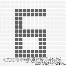
Let's find two pictures img1.png,img2.png, One is a number 6, One is a number 8, Put the two pictures in the same level directory of the code , Verify the recognition effect .
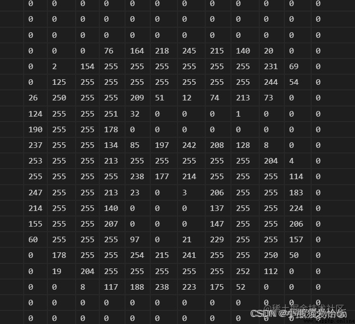
The picture should pass cv2.imread(‘img1.png’,0) Into a two-dimensional array structure ,0 The parameter is grayscale image . After treatment , The array of images is as follows (24,24) Structure :
We need to verify both figures at the same time , So make up the two pictures imgs Put it together ,imgs The structure of is (2,24,24).
 Here's how to build the model , Then load the weights . By calling predicts = model.predict(imgs) take imgs Pass it to the model for prediction and get predicts.
predicts The structure of is (2,15), The values are shown below :
[[ 16.134243 -12.10675 -1.1994154 -27.766754 -43.4324 -9.633694 -12.214878 1.6287893 2.562174 3.2222707 13.834648 28.254173 -6.102874 16.76582 7.2586184] [ 5.022571 -8.762314 -6.7466817 -23.494259 -30.170597 2.4392672 -14.676962 5.8255725 8.855118 -2.0998626 6.820853 7.6578817 1.5132296 24.4664 2.4192357]]
It means yes 2 A prediction , The prediction results of each picture are 15 Maybe .
And then according to index = np.argmax(predict) Find the largest possible index .
Find the numeric value of the character according to the index, and the result is [‘6’, ‘8’].
The following is the monitoring of data in memory :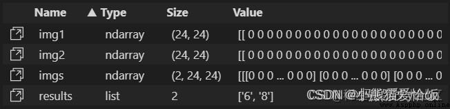 so , Our prediction is accurate .
below , We're going to cut out the numbers in the picture , Identified .
We prepared the data before , Trained data , And take the picture to identify , The recognition result is correct .
up to now , It doesn't seem to be a big problem …… No big problem , It's no big deal to have a problem .
The following is to cut and recognize the picture .
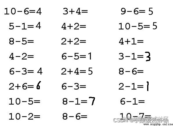 Here's a big picture , How to do it , Make a picture of a single small number .
God said to have light , There's light .
therefore , When the light comes , There is a shadow behind the object .
We'll see , Where there is a shadow, there is something , Where there is no shadow, it is blank .
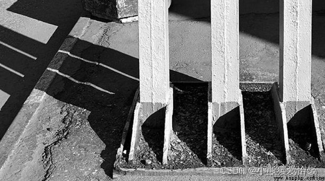 This is projection .
This simple truth is also very practical in image cutting .
Let's make a projection of the pixels of the text , In this way, we can know whether there is text in a certain interval , And know whether the text in this interval is concentrated .
Here is the schematic diagram :
The most effective way , It is often implemented in a loop .
To calculate the projection , You have to count pixel by pixel , See how many pixels , Then record this line with N Pixels . So circular .
 First import the package :
import numpy as np
import cv2
from PIL import Image, ImageDraw, ImageFont
import PIL
import matplotlib.pyplot as plt
import os
import shutil
from numpy.core.records import array
from numpy.core.shape_base import block
import time
For example, it depends on the projection in the vertical direction , The code is as follows :
# Of the whole picture Y Axial projection , Pass in the image array , The picture is binarized and reversed
def img\_y\_shadow(img\_b):
### Computational projection ###
(h,w)=img_b.shape
# Initialize an array with the same length as the height of the image , Used to record the number of black spots in each line
a=[0 for z in range(0,h)]
# Traverse each column , Record how many valid pixels this column contains
for i in range(0,h):
for j in range(0,w):
if img_b[i,j]==255:
a[i]+=1
return a
The final result is such a structure :[0, 79, 67, 50, 50, 50, 109, 137, 145, 136, 125, 117, 123, 124, 134, 71, 62, 68, 104, 102, 83, 14, 4, 0, 0, 0, 0, 0, 0, 0, 0, 0, ……38, 44, 56, 106, 97, 83, 0, 0, 0, 0, 0, 0, 0] Indicates the total number of pixels in the row , The first 1 Line is 0, It means blank white paper , The first 2 Yes 79 Pixels .
What if we want to present it visually ? Then you can stand it up and draw it straight .
# Show pictures
def img\_show\_array(a):
plt.imshow(a)
plt.show()
# Show the projection , Input parameters arr Is a two-dimensional array of pictures ,direction yes x,y Axis
def show\_shadow(arr, direction = 'x'):
a_max = max(arr)
if direction == 'x': # x The projection in the axial direction
a_shadow = np.zeros((a_max, len(arr)), dtype=int)
for i in range(0,len(arr)):
if arr[i] == 0:
continue
for j in range(0, arr[i]):
a_shadow[j][i] = 255
elif direction == 'y': # y The projection in the axial direction
a_shadow = np.zeros((len(arr),a_max), dtype=int)
for i in range(0,len(arr)):
if arr[i] == 0:
continue
for j in range(0, arr[i]):
a_shadow[i][j] = 255
img_show_array(a_shadow)
Let's test the effect :
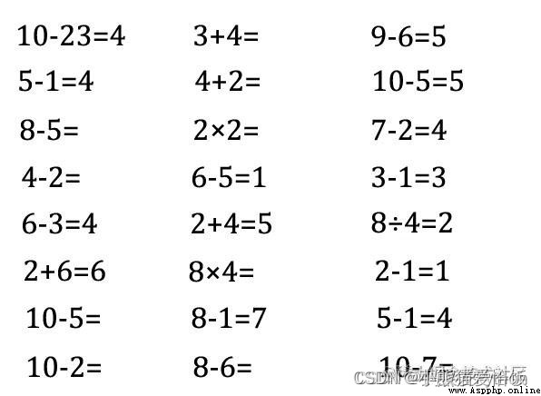
We named the original picture above question.jpg Put it in the code sibling Directory .
# Read in the picture
img_path = 'question.jpg'
img=cv2.imread(img_path,0)
thresh = 200
# Binarization and color reversal
ret,img_b=cv2.threshold(img,thresh,255,cv2.THRESH_BINARY_INV)
The change after binarization and color reversal is as follows :
 The above operation is very useful , Through binarization , Filter out the speckles , Swap black and white by reversing colors , The original white paper area is 255, Now black is 0, More conducive to calculation .
Calculate the projection and show the code :
img_y_shadow_a = img_y_shadow(img_b)
show_shadow(img_y_shadow_a, 'y') # If you want to display the projection
The picture below is the picture above Y The projection on the axis 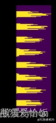 Visually , Basically, you can tell which line is which line .
The most effective way , Often you have to use loops to achieve .
The picture projected above , How do you calculate where to where is a line , Although visible to the naked eye , But computers need rules and algorithms .
# Picture get text block , Pass in the projection list , Returns the array area coordinates of the tag [[ Left , On , Right , Next ]]
def img2rows(a,w,h):
### Partition blocks according to projection ###
inLine = False # Whether the segmentation has started
start = 0 # The starting index of a segmentation
mark_boxs = []
for i in range(0,len(a)):
if inLine == False and a[i] > 10:
inLine = True
start = i
# Record the selected area [ Left , On , Right , Next ], Up and down are pictures , Right and left are start To the current
elif i-start >5 and a[i] < 10 and inLine:
inLine = False
if i-start > 10:
top = max(start-1, 0)
bottom = min(h, i+1)
box = [0, top, w, bottom]
mark_boxs.append(box)
return mark_boxs
By projecting , Calculate which areas are continuous within a certain range , If it lasts for a long time , We think it's the same area , If disconnected for a long time , We think it's another area .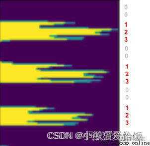 Through this operation , We can get Y The coordinates of the upper and lower boundary points of a row on the axis , Combined with the picture width , In fact, we know the coordinates of the four vertices of a line of pictures mark_boxs What's left is [ sit , On , Right , Next ].
 If you call the following code :
(img_h,img_w)=img.shape
row_mark_boxs = img2rows(img_y_shadow_a,img_w,img_h)
print(row_mark_boxs)
What we get is the coordinates of all the recognized images in each line , This is the format :[[0, 26, 596, 52], [0, 76, 596, 103], [0, 130, 596, 155], [0, 178, 596, 207], [0, 233, 596, 259], [0, 282, 596, 311], [0, 335, 596, 363], [0, 390, 596, 415]]
The most effective way , Finally, it has to be realized by loop . This is also where the computer embodies its power .
# Cut the picture ,img Image array , mark\_boxs Area markers
def cut\_img(img, mark\_boxs):
img_items = [] # Store cropped pictures
for i in range(0,len(mark_boxs)):
img_org = img.copy()
box = mark_boxs[i]
# Cut the picture
img_item = img_org[box[1]:box[3], box[0]:box[2]]
img_items.append(img_item)
return img_items
This step is to hold the box , Draw the small picture from the large picture with a knife , The core code is img_org[box[1]:box[3], box[0]:box[2]] Image clipping , The parameter is an array [ On : Next , Left : Right ], The data obtained is still a two-dimensional array .
If it's preserved :
# Save the picture
def save_imgs(dir_name, imgs):
if os.path.exists(dir_name):
shutil.rmtree(dir_name)
if not os.path.exists(dir_name):
os.makedirs(dir_name)
img_paths = []
for i in range(0,len(imgs)):
file_path = dir_name+'/part\_'+str(i)+'.jpg'
cv2.imwrite(file_path,imgs[i])
img_paths.append(file_path)
return img_paths
# Cut and save
row_imgs = cut\_img(img, row_mark_boxs)
imgs = save\_imgs('rows', row_imgs) # If you want to save the cut
print(imgs)
The picture is like this :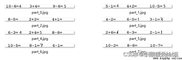
Or cycle? . Walking sideways, we have mastered , So for each line of pictures , Can we cut it into three pieces vertically , A truth . It should be noted that , There is a slight difference between vertical and horizontal , Here is the image above x Axial projection .
 When it's horizontal , There is a gap between words , Then there are gaps between blocks , The degree of this gap needs to be mastered , In order to better distinguish between the spacing of words and the spacing of formula blocks .
fortunately , There is a method called expansion .
Inflation is not positive for people , But for technology , Whether it's inflation (dilate), Or corrosion (erode), As long as the goal can be achieved , All good. .
kernel=np.ones((3,3),np.uint8) # Swelling core size
row\_img\_b=cv2.dilate(img_b,kernel,iterations=6) # Image expansion 6 Time
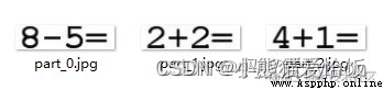
Expand and then project , It's a good way to distinguish . After clipping according to the projection, as shown in the following figure :
 Empathy , No expansion can intercept a single character .
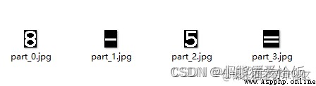 such , This is the character of an area .
A line of , One page , Through the loop , Can be intercepted .
With pictures , You can recognize . With a place , Then we can judge the relationship between the recognition results .
Here are some codes , These codes are incomplete , Some functions you may not find , But ideas can refer to , Detailed code can go to my github Go and see .
def divImg(img\_path, save_file = False):
img_o=cv2.imread(img_path,1)
# Read in the picture
img=cv2.imread(img_path,0)
(img_h,img_w)=img.shape
thresh = 200
# Binarize the whole graph , For branches
ret,img_b=cv2.threshold(img,thresh,255,cv2.THRESH_BINARY_INV)
# Computational projection , And intercept the line of the whole picture
img_y_shadow_a = img_y_shadow(img_b)
row_mark_boxs = img2rows(img_y_shadow_a,img_w,img_h)
# Cut line pictures , Cut is the original picture
row_imgs = cut_img(img, row_mark_boxs)
all_mark_boxs = []
all_char_imgs = []
# =============== Cut from line ======================
for i in range(0,len(row_imgs)):
row_img = row_imgs[i]
(row_img_h,row_img_w)=row_img.shape
# Binary one line graph , Used to cut into pieces
ret,row_img_b=cv2.threshold(row_img,thresh,255,cv2.THRESH_BINARY_INV)
kernel=np.ones((3,3),np.uint8)
# Image expansion 6 Time
row_img_b_d=cv2.dilate(row\_img\_b,kernel,iterations=6)
img_x_shadow_a = img_x_shadow(row_img_b_d)
block\_mark\_boxs = row2blocks(img_x_shadow_a, row_img_w, row_img_h)
row_char_boxs = []
row_char_imgs = []
# Cut into pieces , Cut is the original picture
block\_imgs = cut_img(row_img, block\_mark\_boxs)
if save_file:
b\_imgs = save_imgs('cuts/row\_'+str(i), block\_imgs) # If you want to save the cut
print(b\_imgs)
# ============= Cut words from blocks ====================
for j in range(0,len(block\_imgs)):
block\_img = block\_imgs[j]
(block\_img\_h,block\_img\_w)=block\_img.shape
# Binarization block , Because you have to cut the character picture
ret,block\_img\_b=cv2.threshold(block\_img,thresh,255,cv2.THRESH\_BINARY\_INV)
block\_img\_x\_shadow\_a = img_x_shadow(block\_img\_b)
row_top = row_mark_boxs[i][1]
block\_left = block\_mark\_boxs[j][0]
char_mark_boxs,abs_char_mark_boxs = block2chars(block\_img\_x\_shadow\_a, block\_img\_w, block\_img\_h,row\_top,block\_left)
row_char_boxs.append(abs_char_mark_boxs)
# Cut is a binary graph
char_imgs = cut_img(block\_img\_b, char_mark_boxs, True)
row_char_imgs.append(char_imgs)
if save_file:
c_imgs = save_imgs('cuts/row\_'+str(i)+'/blocks\_'+str(j), char_imgs) # If you want to save the cut
print(c_imgs)
all_mark_boxs.append(row_char_boxs)
all_char_imgs.append(row_char_imgs)
return all_mark_boxs,all_char_imgs,img_o
Fold
The last value returned is 3 individual ,all_mark_boxs Is the coordinate set of the character position of the mark .[ Left , On , Right , Next ] It refers to the coordinates of a character in a large picture , Print it. It's like this :
[[[[19, 26, 34, 53], [36, 26, 53, 53], [54, 26, 65, 53], [66, 26, 82, 53], [84, 26, 101, 53], [102, 26, 120, 53], [120, 26, 139, 53]], [[213, 26, 229, 53], [231, 26, 248, 53], [249, 26, 268, 53], [268, 26, 285, 53]], [[408, 26, 426, 53], [427, 26, 437, 53], [438, 26, 456, 53], [456, 26, 474, 53], [475, 26, 492, 53]]], [[[20, 76, 36, 102], [38, 76, 48, 102], [50, 76, 66, 102], [67, 76, 85, 102], [85, 76, 104, 102]], [[214, 76, 233, 102], [233, 76, 250, 102], [252, 76, 268, 102], [270, 76, 287, 102]], [[411, 76, 426, 102], [428, 76, 445, 102], [446, 76, 457, 102], [458, 76, 474, 102], [476, 76, 493, 102], [495, 76, 511, 102]]]]
It's structured . Its structure is :
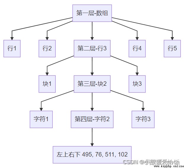 all_char_imgs This return value , Inside is the picture of the corresponding position of the above coordinate structure .img_o It's the original picture .
loop , loop , Or cycle? !
For identifying ,2.3 The forecast data have been talked about , That time was for 2 Recognition of individual pictures , Now we need to identify the small graph set after the whole large graph is segmented , This again uses a loop .
Cui Hua , Code up !
all_mark_boxs,all_char_imgs,img_o = divImg(path,save)
model = cnn.create_model()
model.load_weights('checkpoint/char\_checkpoint')
class_name = np.load('class\_name.npy')
# Traversal line
for i in range(0,len(all_char_imgs)):
row_imgs = all_char_imgs[i]
# Traversal block
for j in range(0,len(row_imgs)):
block_imgs = row_imgs[j]
block_imgs = np.array(block_imgs)
results = cnn.predict(model, block_imgs, class_name)
print('recognize result:',results)
What the above code does is take the block as the unit , Pass it to neural network for prediction , And then return the recognition result .
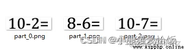
For this picture , Let's cut and recognize .
 Look at the last line at the bottom
recognize result: ['1', '0', '12', '2', '10']
recognize result: ['8', '12', '6', '10']
recognize result: ['1', '0', '12', '7', '10']
The result is an index , Not real characters , According to the dictionary 10: ‘=’, 11: ‘+’, 12: ‘-’, 13: ‘×’, 14: '÷’ After the conversion, the result is :
recognize result: ['1', '0', '-', '2', '=']
recognize result: ['8', '-', '6', '=']
recognize result: ['1', '0', '-', '7', '=']
It corresponds to the picture :
loop ……
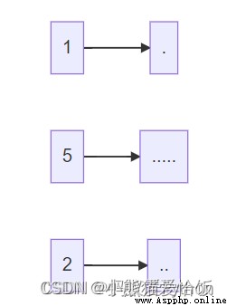
We've got 10-2=、8-6=2, Also get their position coordinates in the original map [ Left , On , Right , Next ], So how to feed back the results to the original map ?
Often there is only the last step left here .
Go over it again : Right , Can make a right sign ; Do wrong , Can cross ; What you didn't do , Can you fill in the answer .
There are two steps to realize : Calculation ( Is it right or wrong ) And feedback ( Write the expected results on the original drawing ).
python There is a powerful function , Namely eval function , Can calculate string expressions , For example, direct calculation eval(“5+3-2”).
therefore , Everything depends on it .
# Calculate the value and return the result Parameters chars:['8', '-', '6', '=']
def calculation(chars):
cstr = ''.join(chars)
result = ''
if("=" in cstr): # There's an equal sign
str_arr = cstr.split('=')
c_str = str_arr[0]
r_str = str_arr[1]
c_str = c_str.replace("×","*")
c_str = c_str.replace("÷","/")
try:
c_r = int(eval(c_str))
except Exception as e:
print("Exception",e)
if r_str == "":
result = c_r
else:
if str(c_r) == str(r_str):
result = "√"
else:
result = "×"
return result
The result obtained after execution is :
recognize result: ['8', '×', '4', '=']
calculate result: 32
recognize result: ['2', '-', '1', '=', '1']
calculate result: √
recognize result: ['1', '0', '-', '5', '=']
calculate result: 5
With the results , Write the results on the picture , This is the last step , It's also the simplest step .
But it works , It's incredibly cumbersome .
You have to find the coordinates , You have to calculate the position of the result , We also want to mark different colors , For example, by the way, it's green , Wrong, it's red , The supplementary answer is gray .
The following code is in a diagram img On , Put the text content text Draw to (left,top) Location , In a specific color and size .
# Draw text
def cv2ImgAddText(img, text, left, top, textColor=(255, 0, 0), textSize=20):
if (isinstance(img, np.ndarray)): # Determine whether OpenCV Picture type
img = Image.fromarray(cv2.cvtColor(img, cv2.COLOR_BGR2RGB))
# Create an object that can be drawn on a given image
draw = ImageDraw.Draw(img)
# The format of the font
fontStyle = ImageFont.truetype("fonts/fangzheng\_shusong.ttf", textSize, encoding="utf-8")
# Draw text
draw.text((left, top), text, textColor, font=fontStyle)
# Convert back to OpenCV Format
return cv2.cvtColor(np.asarray(img), cv2.COLOR_RGB2BGR)
Combined with the information of the cut picture 、 Calculated information , The following code provides ideas and references :
# Get tangent annotation , Cut picture , Original picture
all_mark_boxs,all_char_imgs,img_o = divImg(path,save)
# Recovery model , For image recognition
model = cnn.create_model()
model.load_weights('checkpoint/char\_checkpoint')
class_name = np.load('class\_name.npy')
# Traversal line
for i in range(0,len(all_char_imgs)):
row_imgs = all_char_imgs[i]
# Traversal block
for j in range(0,len(row_imgs)):
block_imgs = row_imgs[j]
block_imgs = np.array(block_imgs)
# Image recognition
results = cnn.predict(model, block_imgs, class_name)
print('recognize result:',results)
# The result of the calculation is
result = calculation(results)
print('calculate result:',result)
# Get the dimension coordinates of the block
block_mark = all_mark_boxs[i][j]
# Get the coordinates of the result , Write in the last word of the block
answer_box = block_mark[-1]
# Calculate the position of the last word
x = answer_box[2]
y = answer_box[3]
iw = answer_box[2] - answer_box[0]
ih = answer_box[3] - answer_box[1]
# Calculate font size
textSize = max(iw,ih)
# Set the font color according to the result
if str(result) == "√":
color = (0, 255, 0)
elif str(result) == "×":
color = (255, 0, 0)
else:
color = (192, 192,192)
# Write the results on the original diagram
img_o = cv2ImgAddText(img_o, str(result), answer_box[2], answer_box[1],color, textSize)
# Save the original drawing filled with results
cv2.imwrite('result.jpg', img_o)
Fold
It turns out that :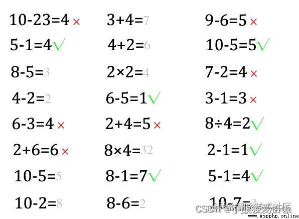
It's the end of the term , Summer vacation is coming again , Is this the happiest thing for everyone . The article shared today is very long , But in such a big project as the end of the term , It is very fragrant to use , I wish you all a happy summer vacation in advance , This is the end of today's article ,