Classification algorithm :C4.5, Naive Bayes (Naive Bayes),SVM,KNN,Adaboost,CARTl . clustering algorithm :K-Means,EMl . Correlation analysis :Aprioril . Connection analysis :PageRank
We use iris as test data to compare the performance of each algorithm .
International authoritative academic organization ICDM (the IEEE International Conference on Data Mining) Ten classic algorithms were selected . For different purposes , I can divide these algorithms into four categories .
Classification algorithm :C4.5(ID3), Naive Bayes (Naive Bayes),SVM,KNN,Adaboost,CARTl ,randomForest,bugging
clustering algorithm :K-Means,EMl
Correlation analysis :Aprioril
Connection analysis :PageRank
C4.5 Is the algorithm of decision tree , It creatively prunes the decision tree in the construction process , And can handle continuous attributes , It can also process incomplete data . It can be said to be in decision tree classification , Algorithm with milestone significance .
Information entropy (entropy) The concept of , It represents the uncertainty of information .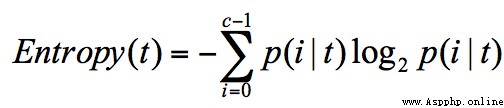
ID3 The algorithm calculates the information gain , Information gain refers to the increase in purity that can be brought about by partitioning , The drop in entropy of information . Its formula , Is the information entropy of the parent node minus the information entropy of all child nodes . In the process of calculation , We will calculate the normalized information entropy of each child node , That is, according to the probability that each child node appears in the parent node , To calculate the information entropy of these child nodes . So the formula of information gain can be expressed as :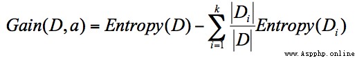
In the formula D It's the father node ,Di Is a child node ,Gain(D,a) Medium a As D Attribute selection of node .
ID3 The node with the largest information gain should be regarded as the parent node , In this way, a decision tree with high purity can be obtained , So we take the node with the greatest information gain as the root node .ID3 The algorithm rules are relatively simple , Strong explanatory ability . There are also defects , For example, we will find ID3 The algorithm tends to select attributes with more values .
ID3 One drawback is , Some attributes may not be very useful for classification tasks , But they may still be chosen as the optimal attribute .
C4.5 What improvements have been made in ID3 Well ?
C4.5 Use information gain rate to select attributes . Information gain rate = Information gain / Attribute entropy .
ID3 When constructing a decision tree , It is easy to produce over fitting . stay C4.5 in , Pessimistic pruning will be used after the decision tree is constructed (PEP), This can improve the generalization ability of the decision tree . Pessimistic pruning is one of the post pruning techniques , The classification error rate of each internal node is estimated recursively , Compare the classification error rate of this node before and after pruning to determine whether to prune it . This pruning method no longer requires a separate test data set .
For incomplete data sets ,C4.5 It can also be processed .
C4.5 You need to scan the dataset multiple times , The algorithm efficiency is relatively low .
Code :
from sklearn import tree
from sklearn.datasets import load_iris
from sklearn.model_selection import train_test_split
X,y = load_iris(return_X_y=True)
train_X,test_X,train_y,test_y = train_test_split(X,y,test_size=0.33,random_state=0)
clf = tree.DecisionTreeClassifier(criterion="entropy")
clf = clf.fit(train_X,train_y)
print(clf.score(test_X,test_y))
Accuracy rate :96%
When the Gini coefficient is smaller , It shows that the difference between samples is small , Low degree of uncertainty . The process of classification itself is a process of reducing uncertainty , That is, the process of improving purity . therefore CART When the algorithm constructs the classification tree , The attribute with the smallest Gini coefficient will be selected as the attribute partition .
GINI Calculation formula of coefficient :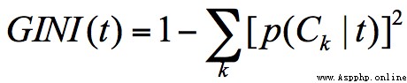
node D The Gini coefficient of is equal to the child node D1 and D2 The sum of the normalized Gini coefficients of , Expressed as :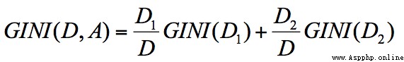
from sklearn import tree
from sklearn.datasets import load_iris
from sklearn.model_selection import train_test_split
X,y = load_iris(return_X_y=True)
train_X,test_X,train_y,test_y = train_test_split(X,y,test_size=0.33,random_state=0)
clf = tree.DecisionTreeClassifier(criterion="gini")
clf = clf.fit(train_X,train_y)
print(clf.score(test_X,test_y))
Accuracy rate :96%
SVM In Chinese, it is called support vector machine , English is Support Vector Machine, abbreviation SVM.SVM A hyperplane classification model is established in the training .
There can be multiple optimal decision surfaces , They all separate data sets correctly , The classification intervals of these optimal decision surfaces may be different , And that has “ The largest interval ”(max margin) The decision-making side of SVM The best solution to find .
nonlinear SVM in , The choice of kernel function affects SVM The biggest variable . The most commonly used kernel functions are linear kernels 、 Polynomial kernel 、 Gaussian kernel 、 Laplace core 、sigmoid nucleus , Or a combination of these kernel functions . The difference between these functions lies in the way they are mapped . Through these kernel functions , We can project the sample space into a new high-dimensional space .
SVM The main idea is hard spacing 、 Soft interval and kernel function .
kernel Represents the choice of kernel functions , It has four options , But the default is rbf, The Gaussian kernel function .
linear: Linear kernel function
poly: Polynomial kernel function
rbf: Gaussian kernel ( Default )
sigmoid:sigmoid Kernel function these four functions represent different ways of mapping , How to choose this 4 The kernel function ?
Linear kernel function , It is used when the data is linearly separable , It's fast , The effect is good . The drawback is that it can't deal with linearly nonseparable data .
Polynomial kernel function can map data from low dimensional space to high dimensional space , But there are many parameters , Large amount of computation .
Gaussian kernel function can also map samples to high-dimensional space , However, compared with polynomial kernel function, it requires less parameters , Usually good performance , So it is the default kernel function .
Students who understand deep learning should know sigmoid It is often used in the mapping of neural networks . Therefore, when choosing sigmoid Kernel function time ,SVM The realization is a multilayer neural network .
from sklearn import svm
from sklearn.datasets import load_iris
from sklearn.model_selection import train_test_split
from sklearn.preprocessing import StandardScaler
X,y = load_iris(return_X_y=True)
train_X,test_X,train_y,test_y = train_test_split(X,y,test_size=0.33,random_state=0)
# use Z-Score Standardize data , Ensure that the data mean of each feature dimension is 0, The variance of 1
ss = StandardScaler()
train_X = ss.fit_transform(train_X)
test_X = ss.transform(test_X)
clf = svm.SVC(kernel='rbf')
clf = clf.fit(train_X,train_y)
print(clf.score(test_X,test_y))
Accuracy rate 96%.
KNN Also called K Nearest neighbor algorithm , English is K-Nearest Neighbor. So-called K a near neighbor , That is, each sample can use its closest K A neighbor represents . If a sample , its K The closest neighbors belong to the classification A, So this sample also belongs to classification A.
KNN How it works . The whole calculation process is divided into three steps :
Calculate the distance between the object to be classified and other objects ;
Count the nearest K A neighbor ;
about K The nearest neighbor , Which category do they belong to the most , What kind of objects do you want to classify .
The idea of cross validation is , Take most of the samples in the sample set as the training set , The remaining small sample is used for prediction , To verify the accuracy of the classification model . So in KNN In the algorithm, , We usually put K Values are selected in a smaller range , At the same time, the one with the highest accuracy on the verification set is finally determined as K value .
KNN Algorithm is one of the simplest algorithms in machine learning , But the project implementation , If the training sample is too large , Then the traditional traversal of the whole sample to find k The nearest neighbor approach will lead to a sharp decline in performance . therefore , To optimize efficiency , Different training data storage structures are incorporated into the implementation . stay sikit-learn Medium KNN Algorithm parameters also provide ’kd_tree’ And so on .
n_neighbors: The default is 5, Namely k-NN Of k Value , Pick the nearest k A little bit .
weights: The default is uniform, Parameters can be uniform、distance
from sklearn.neighbors import KNeighborsClassifier
from sklearn.datasets import load_iris
from sklearn.model_selection import train_test_split
from sklearn.preprocessing import StandardScaler
X,y = load_iris(return_X_y=True)
train_X,test_X,train_y,test_y = train_test_split(X,y,test_size=0.33,random_state=0)
# use Z-Score Standardize data , Ensure that the data mean of each feature dimension is 0, The variance of 1
ss = StandardScaler()
train_X = ss.fit_transform(train_X)
test_X = ss.transform(test_X)
clf = KNeighborsClassifier(n_neighbors=5,algorithm='kd_tree',weights='uniform')
clf = clf.fit(train_X,train_y)
print(clf.score(test_X,test_y))
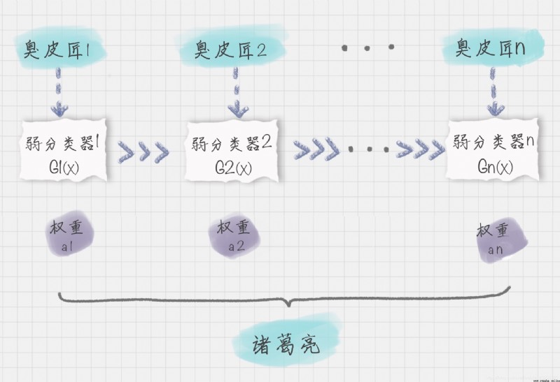
Adaboost A joint classification model is established in the training .boost In English, it means to promote , therefore Adaboost It is a lifting algorithm for constructing classifiers . It allows us to form a strong classifier from multiple weak classifiers , therefore Adaboost It is also a commonly used classification algorithm .
The algorithm trains multiple weak classifiers , Combine them into a strong classifier , That's what we say “ The Three Stooges , Zhuge Liang at the top ”.
Suppose the weak classifier is Gi(x), Its weight in a strong classifier αi, Then we can get a strong classifier f(x):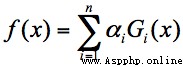
If the classification effect of weak classifier is good , So the weight should be bigger , If the classification effect of weak classifier is general , The weight should be reduced . So we need to determine the weight based on the classification error rate of the weak classifier , It's expressed in terms of the formula :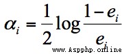
among ei On behalf of the i Classification error rate of classifiers .
AdaBoost The algorithm is realized by changing the data distribution of samples .AdaBoost Will determine whether the samples of each training are correctly classified , For correctly classified samples , Reduce its weight , For samples that are misclassified , Increase its weight . And then based on the last classification accuracy , To determine the weight of each sample in this training sample . Then the new data set with modified weight is passed to the next classifier for training . The advantage of doing so is , Through the dynamic weight of each round of training samples , Can let the training focus on the hard to classify samples , The combination of the final weak classifiers is easier to get higher classification accuracy .
n_estimators: The maximum number of iterations of the algorithm , Is also the number of classifiers , Each iteration will introduce a new weak classifier to increase the combination ability of the original classifier . The default is 50.
from sklearn.ensemble import AdaBoostClassifier
from sklearn.tree import DecisionTreeClassifier
from sklearn.datasets import load_iris
from sklearn.model_selection import train_test_split
from sklearn.preprocessing import StandardScaler
from sklearn.metrics import *
X,y = load_iris(return_X_y=True)
train_X,test_X,train_y,test_y = train_test_split(X,y,test_size=0.33,random_state=0)
# use Z-Score Standardize data , Ensure that the data mean of each feature dimension is 0, The variance of 1
ss = StandardScaler()
train_X = ss.fit_transform(train_X)
test_X = ss.transform(test_X)
clf = AdaBoostClassifier(base_estimator=DecisionTreeClassifier(),n_estimators=50)
clf = clf.fit(train_X,train_y)
pre_y = clf.predict(test_X)
for i,j in zip(pre_y,test_y):
print(i,j)
print('%.4lf'%accuracy_score(pre_y,test_y))
Accuracy rate :96%.
AdaBoost Is a serial combination of multiple weak classifiers , The other is the combination of parallel weak classifiers , It's called Bagging, Stands for random forest .
Apriori Is a kind of mining association rules (association rules) The algorithm of , It does this by mining frequent itemsets (frequent item sets) To reveal the relationship between objects , It is widely used in the fields of business mining and network security . Frequent itemsets are collections of items that often appear together , Association rules imply that there may be a strong relationship between the two objects .
Apriori The algorithm is actually to find frequent itemsets (frequent itemset) The process of . Frequent itemsets are those whose support is greater than or equal to the minimum support (Min Support) Threshold itemset , Therefore, items less than the minimum support are infrequent itemsets , Algorithm to delete , The itemsets with minimum support or greater are frequent itemsets , Then make further division .
Apriori There are several disadvantages in the process of calculation : A large number of candidate sets may be generated . Because of the arrangement and combination , Put together all the possible itemsets ; Each calculation requires rescanning the dataset , To calculate the support of each itemset .
therefore Apriori The algorithm will waste a lot of computing space and time , Therefore, people put forward FP-Growth Algorithm , It is characterized by : Created a tree FP Tree to store frequent itemsets . Delete items that do not meet the minimum support before creation , Reduced storage space . The whole generation process only traverses the data set 2 Time , It greatly reduces the amount of calculation . So in practice , We often use FP-Growth To do frequent itemset mining , Let me give you a brief introduction FP-Growth Principle .
FP It is built according to the frequency of the results , The construction process is as follows :FP-Growth
from efficient_apriori import apriori
data = [[' milk ',' bread ',' diapers '], [' coke ',' bread ', ' diapers ', ' beer '],
[' milk ',' diapers ', ' beer ', ' egg '], [' bread ', ' milk ', ' diapers ',
' beer '], [' bread ', ' milk ', ' diapers ', ' coke ']]
itemsets ,rules = apriori(data,min_support=0.5,min_confidence=1)
print(itemsets)
print(rules)
Output a list of associations :
[{
 milk } -> {
 diapers }, {
 bread } -> {
 diapers }, {
 beer } -> {
 diapers }, {
 milk , bread } -> {
 diapers }]
K-Means Algorithm is a clustering algorithm . I want to divide the object into K class . Suppose that in each category , There was a “ Center point ”, It is the core of this category . Now there is a new point to classify , In this case, just calculate the new point and K The distance between the center points , Which center point is it near , It becomes a category .
K-Means It's unsupervised learning , Randomly assign the center of mass , Then iteratively update the centroid position , Until all points are no longer divided .
from sklearn.preprocessing import StandardScaler
from sklearn.metrics import *
X,y = load_iris(return_X_y=True)
train_X,test_X,train_y,test_y = train_test_split(X,y,test_size=0.33,random_state=0)
# use Z-Score Standardize data , Ensure that the data mean of each feature dimension is 0, The variance of 1
ss = StandardScaler()
train_X = ss.fit_transform(train_X)
test_X = ss.transform(test_X)
clf = KMeans(n_clusters=3,max_iter=300)
clf = clf.fit(train_X,train_y)
pre_y = clf.predict(test_X)
# for i,j in zip(pre_y,test_y):
# print(i,j)
print('%.4lf'%accuracy_score(pre_y,test_y))
Algorithm principle : Using Bayesian formula to calculate the probability of features , That is to use the combination of a priori probability and a posteriori probability , The one with high probability is regarded as the classification result .
Bayes' formula :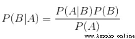
In another way, it will be much clearer , as follows :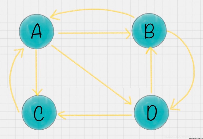
We finally got p( Category | features ) that will do ! And can be transformed into the use of existing data , Calculate a posteriori probability and a priori probability . That is, the statistical information of existing test data samples , You can get p( Category | features ) Value . Detailed explanation
sklearn Machine learning package sklearn The full name of Scikit-learn, It provides us with 3 A naive Bayesian classification algorithm , Gauss naive Bayes (GaussianNB)、 Polynomial naive Bayes (MultinomialNB) And Bernoulli, naive Bayes (BernoulliNB). These three algorithms are suitable for different scenarios , We should choose different algorithms according to different characteristic variables :
Gaussian naive Bayes : Characteristic variables are continuous variables , In line with the Gaussian distribution , For example, people's height , The length of the object .
Polynomial naive Bayes : Characteristic variables are discrete variables , According to the multinomial distribution , In document classification, the characteristic variable is reflected in the number of times a word appears , Or words TF-IDF It's worth waiting for .
Bernoulli naive Bayes : Characteristic variables are Boolean variables , accord with 0/1 Distribution , In document classification, the feature is whether words appear .
Naive Bayesian model is based on the principle of probability theory , Its idea is like this : Want to classify the given unknown objects , It is necessary to solve the probability of each category under the condition that the unknown object appears , Which is the biggest , It is considered that this unknown object belongs to which category .
Bayesian principle 、 There is a difference between Bayesian classification and naive Bayes : Bayesian principle is the biggest concept , It solves the problem of “ Reverse probability ” The problem of , Based on this theory , Bayesian classifier has been designed , Naive Bayesian classification is one of Bayesian classifiers , It's also the simplest , The most commonly used classifier .
Naive Bayes is naive because it assumes that attributes are independent of each other , Therefore, there are constraints on the actual situation , If there is an association between attributes , The classification accuracy will be reduced . But for the most part , Naive Bayes classification results are good .
Naive Bayes classification is often used in text classification , Especially for English and other languages , The classification effect is very good . It is often used for spam text filtering 、 Emotional prediction 、 Recommendation system, etc .
from sklearn.naive_bayes import MultinomialNB
from sklearn.datasets import load_iris
from sklearn.model_selection import train_test_split
X,y = load_iris(return_X_y=True)
train_X,test_X,train_y,test_y = train_test_split(X,y,test_size=0.33,random_state=0)
clf = MultinomialNB(alpha=0.001)
clf = clf.fit(train_X,train_y)
print(clf.score(test_X,test_y))
Accuracy rate 70%. Using polynomial Bayes .
If we use Gaussian Bayes :
from sklearn.naive_bayes import MultinomialNB,GaussianNB
clf = GaussianNB()
Accuracy rate 96%.
EM English is Expectation Maximization, therefore EM Algorithm is also called maximum expectation algorithm ., It is a method to find the maximum likelihood estimation of parameters .
The principle is : Suppose we want to evaluate parameters A And parameters B, In the initial state, both are unknown , And got it A You can get B Information about , In turn, I know B And you get A. Consider giving... First A Some initial value , So as to get B Valuation of , And then from B Starting from the valuation of , Reevaluate A The value of , This process continues until convergence .EM Algorithms are often used in clustering and machine learning .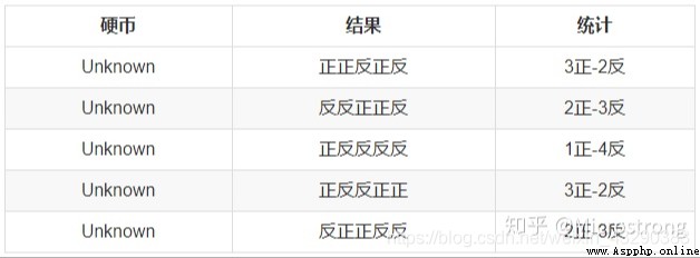
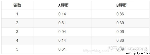
First , Random selection PA= positive PB = positive The initial value of the .EM Algorithm E step , Is calculated under the current estimated parameters , Implied variables ( yes A Or coins B COINS ) The probability of occurrence of each value of , The seat with the maximum probability is A still B.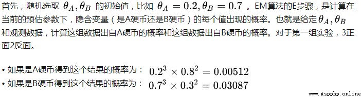
from sklearn.mixture import GaussianMixture
from sklearn.datasets import load_iris
from sklearn.model_selection import train_test_split
from sklearn.preprocessing import StandardScaler
from sklearn.metrics import *
X,y = load_iris(return_X_y=True)
train_X,test_X,train_y,test_y = train_test_split(X,y,test_size=0.33,random_state=0)
# use Z-Score Standardize data , Ensure that the data mean of each feature dimension is 0, The variance of 1
ss = StandardScaler()
train_X = ss.fit_transform(train_X)
test_X = ss.transform(test_X)
clf = GaussianMixture(n_components=3)
clf = clf.fit(train_X,train_y)
pre_y = clf.predict(test_X)
# for i,j in zip(pre_y,test_y):
# print(i,j)
print('%.4lf'%accuracy_score(pre_y,test_y))
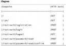
PageRank It originated from the calculation of the influence of the paper , If a literary theory is introduced more times , It means that the stronger the influence of this paper . Again PageRank By Google It is creatively applied to the calculation of web page weight : When a page chains out more pages , Description of this page “ reference ” The more , The more frequently this page is linked , The higher the number of times this page is referenced . Based on this principle , We can get the weight of the website .
Let's say there are 4 Pages A、B、C、D. The link information between them is as shown in the figure :
The influence of a web page = The sum of the weighted influence of all pages in the chain collection , Expressed as :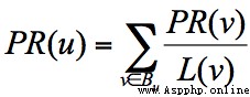
In the example , You can see A There are three outbound links to B、C、D On . Then when the user accesses A When , There's a jump to B、C perhaps D The possibility of , Jump probability is 1/3.B There are two out of the chain , Linked to A and D On , The jump probability is 1/2. such , We can get A、B、C、D Transfer matrix of these four web pages M: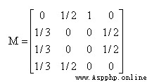
hypothesis A、B、C、D The initial impact of all four pages is the same , namely :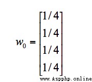
After the first transfer , Influence of each page w1 Turn into :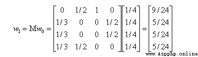
And then we multiply that by the transfer matrix w1 obtain w2 result , Until the first n After iterations wn Influence is no longer changing , Can converge to (0.3333,0.2222,0.2222,0.2222), Which means A、B、C、D The influence of the final balance of the four pages .
A The weight of the page is greater than other pages , That is to say PR Higher value . and B、C、D Page PR The values are equal .
import networkx as nx
# Create a directed graph
G = nx.DiGraph()
# The relationship between edges of Digraphs
edges = [("A", "B"), ("A", "C"), ("A", "D"), ("B", "A"), ("B", "D"), ("C", "A"), ("D", "B"), ("D", "C")]
for edge in edges:
G.add_edge(edge[0], edge[1])
pagerank_list = nx.pagerank(G, alpha=1)
print("pagerank The value is :", pagerank_list)
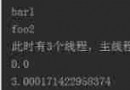
result :
pagerank The value is : {
'A': 0.33333396911621094, 'B': 0.22222201029459634, 'C': 0.22222201029459634, 'D': 0.22222201029459634}
Random forest is the idea of integrated learning : An algorithm that integrates multiple trees in parallel , Its basic unit is the decision tree , And its essence belongs to a big branch of machine learning —— Integrated learning (Ensemble Learning) Method .
There are two key words in the name of random forest , One is “ Random ”, One is “ The forest ”.“ The forest ” It's easy for us to understand , One is called a tree , Then hundreds of trees can be called forests , This analogy is very appropriate , In fact, this is also the main idea of random forest – The embodiment of integration thought .
“ Random ” The meaning is : If the training set size is N, For every tree , Randomly and put back from the training set N Training samples ( This sampling method is called bootstrap sample Method ), As the training set of the tree . Detailed explanation
from sklearn.ensemble import RandomForestClassifier
from sklearn.tree import DecisionTreeClassifier
from sklearn.datasets import load_iris
from sklearn.model_selection import train_test_split
from sklearn.preprocessing import StandardScaler
from sklearn.metrics import *
X,y = load_iris(return_X_y=True)
train_X,test_X,train_y,test_y = train_test_split(X,y,test_size=0.33,random_state=0)
# use Z-Score Standardize data , Ensure that the data mean of each feature dimension is 0, The variance of 1
ss = StandardScaler()
train_X = ss.fit_transform(train_X)
test_X = ss.transform(test_X)
clf = RandomForestClassifier(n_jobs=-1)
clf = clf.fit(train_X,train_y)
pre_y = clf.predict(test_X)
# for i,j in zip(pre_y,test_y):
# print(i,j)
print('%.4lf'%accuracy_score(pre_y,test_y))
Understand the basic algorithm principle , Although it is unlikely that we will implement the algorithm ourselves , It is useful to know the algorithm .
 Pandas Matplotlib solution to the problem of incomplete display caused by too long coordinate axis labels when saving drawings
Catalog Preface 1. Problem de
 Appium+python mobile terminal (Android) automated test environment was not so difficult to build+ Take you to practice
Appium Its a mobile automation