VBA在Excel中的應用（三）

目錄

Chart Export

Chart Format

Chart Lengend

Chart Protect

Chart Title

Chart

Chart Export

1.將Excel中的圖表導出成gif格式的圖片保存到硬盤上

Sub ExportChart()
Dim myChart As Chart
Set myChart=ActiveChart
myChart.Export Filename:="C:\Chart.gif", Filtername:="GIF"
End Sub

理論上圖表可以被保存成任何類型的圖片文件，讀者可以自己去嘗試。

2.將Excel中的圖表導出成可交互的頁面保存到硬盤上

Sub SaveChartWeb()
ActiveWorkbook.PublishObjects.Add _
SourceType:=xlSourceChart, _
Filename:=ActiveWorkbook.Path &　"\Sample2.htm", _
Sheet:=ActiveSheet.name, _
Source:=" Chart 1", _
HtmlType:=xlHtmlChart

ActiveWorkbook.PublishObjects(1).Publish (True)
End Sub

Chart Format

1.操作Chart對象。給幾個用VBA操作Excel Chart對象的例子，讀者可以自己去嘗試一下。

Public　Sub ChartInterior()
Dim myChart As Chart
'Reference embedded chart
Set myChart=ActiveSheet.ChartObjects(1).Chart
With myChart　　 'Alter interior colors of chart components
.ChartArea.Interior.Color=RGB(1, 2, 3)
.PlotArea.Interior.Color=RGB(11, 12, 1)
.Legend.Interior.Color=RGB(31, 32, 33)
If .HasTitle Then
.ChartTitle.Interior.Color=RGB(41, 42, 43)
End　If
End　With
End Sub

Public　Sub SetXAxis()
Dim myAxis As Axis
Set myAxis=ActiveSheet.ChartObjects(1).Chart.Axes(xlCategory, xlPrimary)
With myAxis　　　 'Set properties of x-axis
.HasMajorGridlines=True
.HasTitle=True
.AxisTitle.Text="My Axis"
.AxisTitle.Font.Color=RGB(1, 2, 3)
.CategoryNames=Range("C2:C11")
.TickLabels.Font.Color=RGB(11, 12, 13)
End　With
End Sub

Public　Sub TestSeries()
Dim mySeries As Series
Dim seriesCol As SeriesCollection
Dim I As　Integer
I=1
Set seriesCol=ActiveSheet.ChartObjects(1).Chart.SeriesCollection
For　Each mySeries In seriesCol
Set mySeries=ActiveSheet.ChartObjects(1).Chart.SeriesCollection(I)
With mySeries
.MarkerBackgroundColor=RGB(1, 32, 43)
.MarkerForegroundColor=RGB(11, 32, 43)
.Border.Color=RGB(11, 12, 23)
End　With
I=I +　1
Next
End Sub

Public　Sub TestPoint()
Dim myPoint As Point
Set myPoint=ActiveSheet.ChartObjects(1).Chart.SeriesCollection(1).Points(3)
With myPoint
.ApplyDataLabels xlDataLabelsShowValue
.MarkerBackgroundColor=RGB(1, 2, 3)
.MarkerForegroundColor=RGB(11, 22, 33)
End　With
End Sub

Sub chartAxis()
Dim myChartObject As ChartObject
Set myChartObject=ActiveSheet.ChartObjects.Add(Left:=200, Top:=200, _
Width:=400, Height:=300)

myChartObject.Chart.SetSourceData Source:= _
ActiveWorkbook.Sheets("Chart Data").Range("A1:E5")

myChartObject.SeriesCollection.Add Source:=ActiveSheet.Range("C4:K4"), Rowcol:=xlRows
myChartObject.SeriesCollection.NewSeries
myChartObject.HasTitle=True

With myChartObject.Axes(Type:=xlCategory, AxisGroup:=xlPrimary)
.HasTitle=True
.AxisTitle.Text="Years"
.AxisTitle.Font.Name="Times New Roman"
.AxisTitle.Font.Size=12
.HasMajorGridlines=True
.HasMinorGridlines=False
End　With
End Sub

Sub FormattingCharts()
Dim myChart As Chart
Dim ws As Worksheet
Dim ax As Axis

Set ws=ThisWorkbook.Worksheets("Sheet1")
Set myChart=GetChartByCaption(ws, "GDP")

If　Not myChart Is　Nothing　Then
Set ax=myChart.Axes(xlCategory)
With ax
.AxisTitle.Font.Size=12
.AxisTitle.Font.Color=vbRed
End　With
Set ax=myChart.Axes(xlValue)
With ax
.HasMinorGridlines=True
.MinorGridlines.Border.LineStyle=xlDashDot
End　With
With myChart.PlotArea
.Border.LineStyle=xlDash
.Border.Color=vbRed
.Interior.Color=vbWhite
.Width=myChart.PlotArea.Width +　10
.Height=myChart.PlotArea.Height +　10
End　With
myChart.ChartArea.Interior.Color=vbWhite
myChart.Legend.Position=xlLegendPositionBottom
End　If

Set ax=Nothing
Set myChart=Nothing
Set ws=Nothing
End Sub
Function GetChartByCaption(ws As Worksheet, sCaption As　String) As Chart
Dim myChart As ChartObject
Dim myChart As Chart
Dim sTitle As　String

Set myChart=Nothing
For　Each myChart In ws.ChartObjects
If myChart.Chart.HasTitle Then
sTitle=myChart.Chart.ChartTitle.Caption
If　StrComp(sTitle, sCaption, vbTextCompare)=0　Then
Set myChart=myChart.Chart
Exit　For
End　If
End　If
Next
Set GetChartByCaption=myChart
Set myChart=Nothing
Set myChart=Nothing
End Function

2.使用VBA在Excel中添加圖表

Public　Sub AddChartSheet()
Dim aChart As Chart

Set aChart=Charts.Add
With aChart
.Name="Mangoes"
.ChartType=xlColumnClustered
.SetSourceData Source:=Sheets("Sheet1").Range("A3:D7"), PlotBy:=xlRows
.HasTitle=True
.ChartTitle.Text="=Sheet1!R3C1"
End　With
End Sub

3.遍歷並更改Chart對象中的圖表類型

Sub ChartType()
Dim myChart As ChartObject
For　Each myChart In ActiveSheet.ChartObjects
myChart.Chart.Type=xlArea
Next myChart
End Sub

4.遍歷並更改Chart對象中的Legend

Sub LegendMod()
Dim myChart As ChartObject
For　Each myChart In ActiveSheet.ChartObjects
With myChart.Chart.Legend.font
.name="Calibri"
.FontStyle="Bold"
.Size=12
End　With
Next myChart
End Sub

5.一個格式化Chart的例子

Sub ChartMods()
ActiveChart.Type=xlArea
ActiveChart.ChartArea.font.name="Calibri"
ActiveChart.ChartArea.font.FontStyle="Regular"
ActiveChart.ChartArea.font.Size=9
ActiveChart.PlotArea.Interior.ColorIndex=xlNone
ActiveChart.Axes(xlValue).TickLabels.font.bold=True
ActiveChart.Axes(xlCategory).TickLabels.font.bold=True
ActiveChart.Legend.Position=xlBottom
End Sub

6.通過VBA更改Chart的Title

Sub ApplyTexture()
Dim myChart As Chart
Dim ser As Series
Set myChart=ActiveChart
Set ser=myChart.SeriesCollection(2)
ser.Format.Fill.PresetTextured (msoTextureGreenMarble)
End Sub

7.在VBA中使用自定義圖片填充Chart對象的series區域

Sub FormatWithPicture()
Dim myChart As Chart
Dim ser As Series
Set myChart=ActiveChart
Set ser=myChart.SeriesCollection(1)
MyPic="C:\Title.jpg"
ser.Format.Fill.UserPicture (MyPic)
End Sub

Excel中的Chart允許用戶對其中選定的區域自定義樣式，其中包括使用圖片選中樣式。在Excel的Layout菜單下有一個Format Selection，首先在Chart對象中選定要格式化的區域，例如series，然後選擇該菜單，在彈出的對話框中即可對所選的區域進行格式化。如series選項、填充樣式、邊框顏色和樣式、陰影以及3D效果等。下面再給出一個在VBA中使用漸變色填充Chart對象的series區域的例子。

Sub TwoColorGradient()
Dim myChart As Chart
Dim ser As Series
Set myChart=ActiveChart
Set ser=myChart.SeriesCollection(1)
MyPic="C:\Title1.jpg"
ser.Format.Fill.TwoColorGradient msoGradientFromCorner, 3
ser.Format.Fill.ForeColor.ObjectThemeColor=msoThemeColorAccent6
ser.Format.Fill.BackColor.ObjectThemeColor=msoThemeColorAccent2
End Sub

8.通過VBA格式化Chart對象中series的趨勢線樣式

Sub FormatLineOrBorders()
Dim myChart As Chart
Set myChart=ActiveChart
With myChart.SeriesCollection(1).Trendlines(1).Format.Line
.DashStyle=msoLineLongDashDotDot
.ForeColor.RGB=RGB(50, 0, 128)
.BeginArrowheadLength=msoArrowheadShort
.BeginArrowheadStyle=msoArrowheadOval
.BeginArrowheadWidth=msoArrowheadNarrow
.EndArrowheadLength=msoArrowheadLong
.EndArrowheadStyle=msoArrowheadTriangle
.EndArrowheadWidth=msoArrowheadWide
End　With
End Sub

Excel允許用戶為Chart對象的series添加趨勢線（trendline），首先在Chart中選中要設置的series，然後選擇Layout菜單下的trendline，選擇一種trendline樣式。

9.一組利用VBA格式化Chart對象的例子

Sub FormatBorder()
Dim myChart As Chart
Set myChart=ActiveChart
With myChart.ChartArea.Format.Line
.DashStyle=msoLineLongDashDotDot
.ForeColor.RGB=RGB(50, 0, 128)
End　With
End Sub

Sub AddGlowToTitle()
Dim myChart As Chart
Set myChart=ActiveChart
myChart.ChartTitle.Format.Line.ForeColor.RGB=RGB(255, 255, 255)
myChart.ChartTitle.Format.Line.DashStyle=msoLineSolid
myChart.ChartTitle.Format.Glow.Color.ObjectThemeColor=msoThemeColorAccent6
myChart.ChartTitle.Format.Glow.Radius=8
End Sub

Sub FormatShadow()
Dim myChart As Chart
Set myChart=ActiveChart
With myChart.Legend.Format.Shadow
.ForeColor.RGB=RGB(0, 0, 128)
.OffsetX=5
.OffsetY=-3
.Transparency=0.5
.Visible=True
End　With
End Sub

Sub FormatSoftEdgesWithLoop()
Dim myChart As Chart
Dim ser As Series
Set myChart=ActiveChart
Set ser=myChart.SeriesCollection(1)
For i=1　To　6
ser.Points(i).Format.SoftEdge.Type=i
Next i
End Sub

10.在VBA中對Chart對象應用3D效果

Sub Assign3DPreset()
Dim myChart As Chart
Dim shp As Shape
Set myChart=ActiveChart
Set shp=myChart.Shapes(1)
shp.ThreeD.SetPresetCamera msoCameraIsometricLeftDown
End Sub

Sub AssignBevel()
Dim myChart As Chart
Dim ser As Series
Set myChart=ActiveChart
Set ser=myChart.SeriesCollection(1)
ser.Format.ThreeD.Visible=True
ser.Format.ThreeD.BevelTopType=msoBevelCircle
ser.Format.ThreeD.BevelTopInset=16
ser.Format.ThreeD.BevelTopDepth=6
End Sub

Chart Lengend

1.設置Lengend的位置和ChartArea的顏色

Sub FormattingCharts()
Dim myChart As Chart
Dim ws As Worksheet
Dim ax As Axis

Set ws=ThisWorkbook.Worksheets("Sheet1")
Set myChart=GetChartByCaption(ws, "GDP")

If　Not myChart Is　Nothing　Then
myChart.ChartArea.Interior.Color=vbWhite
myChart.Legend.Position=xlLegendPositionBottom
End　If

Set ax=Nothing
Set myChart=Nothing
Set ws=Nothing
End Sub
Function GetChartByCaption(ws As Worksheet, sCaption As　String) As Chart
Dim myChart As ChartObject
Dim myChart As Chart
Dim sTitle As　String

Set myChart=Nothing
For　Each myChart In ws.ChartObjects
If myChart.Chart.HasTitle Then
sTitle=myChart.Chart.ChartTitle.Caption
If　StrComp(sTitle, sCaption, vbTextCompare)=0　Then
Set myChart=myChart.Chart
Exit　For
End　If
End　If
Next
Set GetChartByCaption=myChart
Set myChart=Nothing
Set myChart=Nothing
End Function

2.通過VBA給Chart添加Lengend

Sub legend()
Dim myChartObject As ChartObject
Set myChartObject=ActiveSheet.ChartObjects.Add(Left:=200, Top:=200, _
Width:=400, Height:=300)

myChartObject.Chart.SetSourceData Source:= _
ActiveWorkbook.Sheets("Chart Data").Range("A1:E5")

myChartObject.SeriesCollection.Add Source:=ActiveSheet.Range("C4:K4"), Rowcol:=xlRows
myChartObject.SeriesCollection.NewSeries
With myChartObject.Legend
.HasLegend=True
.Font.Size=16
.Font.Name="Arial"
End　With
End Sub

Chart Protect

1.保護圖表

Sub ProtectChart()
Dim myChart As Chart
Set myChart=ThisWorkbook.Sheets("Protected Chart")
myChart.Protect "123456", True, True, , True
myChart.ProtectData=False
myChart.ProtectGoalSeek=True
myChart.ProtectSelection=True
End Sub

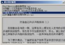
Excel中的Chart可以和Sheet一樣被保護，讀者可以選中圖表所在的Tab，然後通過Review菜單下的Protect Sheet菜單來對圖表進行保護設置。代碼中的Protected Chart123456是設置保護時的密碼，有關Protect函數的參數和設置保護時的其它屬性讀者可以查閱Excel自帶的幫助文檔。

2.取消圖表保護

Sub UnprotectChart()
Dim myChart As Chart
Set myChart=ThisWorkbook.Sheets("Protected Chart")
myChart.Unprotect "123456"
myChart.ProtectData=False
myChart.ProtectGoalSeek=False
myChart.ProtectSelection=False
End Sub

與保護圖表的示例相對應，可以通過VBA撤銷對圖表的保護設置。

Chart Title

1.通過VBA添加圖表的標題

Sub chartTitle()
Dim myChartObject As ChartObject
Set myChartObject=ActiveSheet.ChartObjects.Add(Left:=200, Top:=200, _
Width:=400, Height:=300)

myChartObject.Chart.SetSourceData Source:= _
ActiveWorkbook.Sheets("Chart Data").Range("A1:E5")

myChartObject.SeriesCollection.Add Source:=ActiveSheet.Range("C4:K4"), Rowcol:=xlRows
myChartObject.SeriesCollection.NewSeries
myChartObject.HasTitle=True
End Sub

如果要設置標題顯示的位置，可以在上述代碼的後面加上：

With myChartObject.ChartTitle
.Top=100
.Left=150
End With

如果要同時設置標題字體，可以在上述代碼的後面加上：

myChartObject.ChartTitle.Font.Name="Times"

2.通過VBA修改圖表的標題

Sub charTitleText()
ActiveChart.ChartTitle.Text="Industrial Disease in North Dakota"
End Sub

3.一個通過標題搜索圖表的例子

Function GetChartByCaption(ws As Worksheet, sCaption As　String) As Chart
Dim myChart As ChartObject
Dim myChart As Chart
Dim sTitle As　String

Set myChart=Nothing
For　Each myChart In ws.ChartObjects
If myChart.Chart.HasTitle Then
sTitle=myChart.Chart.ChartTitle.Caption
If　StrComp(sTitle, sCaption, vbTextCompare)=0　Then
Set myChart=myChart.Chart
Exit　For
End　If
End　If
Next
Set GetChartByCaption=myChart
Set myChart=Nothing
Set myChart=Nothing
End Function
Sub TestGetChartByCaption()
Dim myChart As Chart
Dim ws As Worksheet
Set ws=ThisWorkbook.Worksheets("Sheet1")
Set myChart=GetChartByCaption(ws, "I am the Chart Title")

If　Not myChart Is　Nothing　Then
Debug.Print "Found chart"
Else
Debug.Print "Sorry - chart not found"
End　If

Set ws=Nothing
Set myChart=Nothing
End Sub

Chart

通過VBA創建Chart的幾種方式

使用ChartWizard方法創建

Sub CreateExampleChartVersionI()
Dim ws As Worksheet
Dim rgChartData As Range
Dim myChart As Chart

Set ws=ThisWorkbook.Worksheets("Sheet1")
Set rgChartData=ws.Range("B1").CurrentRegion
Set myChart=Charts.Add
Set myChart=myChart.Location(xlLocationAsObject, ws.Name)
With myChart
.ChartWizard _
Source:=rgChartData, _
Gallery:=xlColumn, _
Format:=1, _
PlotBy:=xlColumns, _
CategoryLabels:=1, _
SeriesLabels:=1, _
HasLegend:=True, _
Title:="Version I", _
CategoryTitle:="Year", _
ValueTitle:="GDP in billions of $"
End　With

Set myChart=Nothing
Set rgChartData=Nothing
Set ws=Nothing
End Sub

使用Chart Object方法創建

Sub CreateExampleChartVersionII()
Dim ws As Worksheet
Dim rgChartData As Range
Dim myChart As Chart

Set ws=ThisWorkbook.Worksheets("Basic Chart")
Set rgChartData=ws.Range("B1").CurrentRegion
Set myChart=Charts.Add
Set myChart=myChart.Location(xlLocationAsObject, ws.Name)

With myChart
.SetSourceData rgChartData, xlColumns
.HasTitle=True
.ChartTitle.Caption="Version II"
.ChartType=xlColumnClustered

With .Axes(xlCategory)
.HasTitle=True
.AxisTitle.Caption="Year"
End　With

With .Axes(xlValue)
.HasTitle=True
.AxisTitle.Caption="GDP in billions of $"
End　With

End　With

Set myChart=Nothing
Set rgChartData=Nothing
Set ws=Nothing
End Sub

使用ActiveWorkbook.Sheets.Add方法創建

Sub chart()
Dim myChartSheet As Chart
Set myChartSheet=ActiveWorkbook.Sheets.Add _
(After:=ActiveWorkbook.Sheets(ActiveWorkbook.Sheets.Count), _
Type:=xlChart)
End Sub

使用ActiveSheet.ChartObjects.Add方法創建

Sub charObj()
Dim myChartObject As ChartObject
Set myChartObject=ActiveSheet.ChartObjects.Add(Left:=200, Top:=200, _
Width:=400, Height:=300)
myChartObject.Chart.SetSourceData Source:= _
ActiveWorkbook.Sheets("Chart Data").Range("A1:E5")
End Sub

不同的創建方法可以應用在不同的場合，如Sheet中內嵌的圖表，一個獨立的Chart Tab等，讀者可以自己研究。最後一種方法的末尾給新創建的圖表設定了數據源，這樣圖表就可以顯示出具體的圖形了。

如果需要指定圖表的類型，可以加上這句代碼：

myChartObject.ChartType=xlColumnStacked

如果需要在現有圖表的基礎上添加新的series，下面這行代碼可以參考：

myChartObject.SeriesCollection.Add Source:=ActiveSheet.Range("C4:K4"), Rowcol:=xlRows

或者通過下面這行代碼對已有的series進行擴展：

myChartObject.SeriesCollection.Extend Source:=Worksheets("Chart Data").Range("P3:P8")

2.一個相對完整的通過VBA創建Chart的例子

'Common Excel Chart Types
'-------------------------------------------------------------------
'Chart　　 |　　 VBA Constant (ChartType property of Chart object)　　　　 |
'==================================================================　　　　　　　
'Column　 |　　 xlColumnClustered, xlColumnStacked, xlColumnStacked100|　　　　　　　　
'Bar　　　　 |　　 xlBarClustered, xlBarStacked, xlBarStacked100　　　　　　　　 |
'Line　　　 |　　 xlLine, xlLineMarkersStacked, xlLineStacked　　　　　　　　　　 |
'Pie　　　　 |　　 xlPie, xlPieOfPie　　　　　　　　　　　　　　　　　　　　　　　　　　　　　　　　　　　　 |
'Scatter |　　 xlXYScatter, xlXYScatterLines　　　　　　　　　　　　　　　　　　　　　　　　 |
'-------------------------------------------------------------------

Public　Sub AddChartSheet()
Dim dataRange As Range
Set dataRange=ActiveWindow.Selection
Charts.Add　　 'Create a chart sheet
With ActiveChart　　　 'Set chart properties
.ChartType=xlColumnClustered
.HasLegend=True
.Legend.Position=xlRight

.Axes(xlCategory).MinorTickMark=xlOutside
.Axes(xlValue).MinorTickMark=xlOutside
.Axes(xlValue).MaximumScale=_
Application.WorksheetFunction.RoundUp( _
Application.WorksheetFunction.Max(dataRange), -1)
.Axes(xlCategory).HasTitle=True
.Axes(xlCategory).AxisTitle.Characters.Text="X-axis Labels"
.Axes(xlValue).HasTitle=True
.Axes(xlValue).AxisTitle.Characters.Text="Y-axis"

.SeriesCollection(1).name="Sample Data"
.SeriesCollection(1).Values=dataRange
End　With
End Sub

3.通過選取的Cells Range的值設置Chart中數據標簽的內容

Sub DataLabelsFromRange()
Dim DLRange As range
Dim myChart As Chart
Dim i As　Integer

Set myChart=ActiveSheet.ChartObjects(1).Chart
On　Error　Resume　Next
Set DLRange=Application.InputBox _
(prompt:="Range for data labels?", Type:=8)
If DLRange Is　Nothing　Then　Exit　Sub
On　Error　GoTo　0
myChart.SeriesCollection(1).ApplyDataLabels Type:=xlDataLabelsShowValue, AutoText:=True, LegendKey:=False
Pts=myChart.SeriesCollection(1).Points.Count
For i=1　To Pts
myChart.SeriesCollection(1)._
Points(i).DataLabel.Characters.Text=DLRange(i)
Next i
End Sub

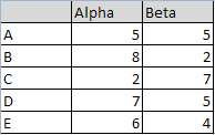
考慮下面這個場景，當采用下表的數據生成圖表Chart4時，默認的效果如下圖。

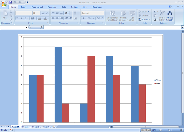
可以手動給該圖表添加Data Labels，方法是選中任意的series，右鍵選擇Add Data Labels。如果想要為所有的series添加Data Labels，則需要依次選擇不同的series，然後重復該操作。

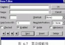
Excel中可以通過VBA將指定Cells Range中的值設置到Chart的Data Labels中，上面的代碼就是一個例子。程序執行的時候會首先彈出一個提示框，要求用戶通過鼠標去選擇一個單元格區域以獲取到Cells集合（或者直接輸入地址），如下圖：

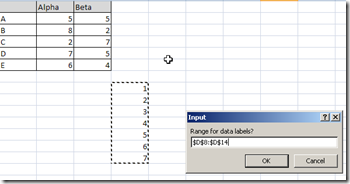
注意VBA中輸入型對話框Application.InputBox的使用。在循環中將Range中的值添加到Chart的Data Labels中。

4.一個使用VBA給Chart添加Data Labels的例子

Sub　AddDataLabels()
Dim　seSales　As　Series
Dim　pts　As　Points
Dim　pt　As　Point
Dim　rngLabels　As　range
Dim　iPointIndex　As　Integer

Set　rngLabels　=　range("B4:G4")

Set　seSales　=　ActiveSheet.ChartObjects(1).Chart.SeriesCollection(1)
seSales.HasDataLabels　=　True

Set　pts　=　seSales.Points

For　Each　pt　In　pts
iPointIndex　=　iPointIndex　+　1
pt.DataLabel.text　=　rngLabels.cells(iPointIndex).text
pt.DataLabel.font.bold　=　True
pt.DataLabel.Position　=　xlLabelPositionAbove
Next　pt
End　Sub