VBA在Excel中的應用（二）

目錄

AutoFilter

Binding

Cell Comments

Cell Copy

Cell Format

Cell Number Format

Cell Value

Cell

AutoFilter

1.確認當前工作表是否開啟了自動篩選功能

Sub　filter()
If ActiveSheet.AutoFilterMode Then
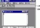
MsgBox　"Turned on"
End　If
End Sub

當工作表中有單元格使用了自動篩選功能，工作表的AutoFilterMode的值將為True，否則為False。

2.使用Range.AutoFilter方法

Sub Test()
Worksheets("Sheet1").Range("A1").AutoFilter _
field:=1, _
Criteria1:="Otis"
VisibleDropDown:=False
End Sub

以上是一段來源於Excel幫助文檔的例子，它從A1單元格開始篩選出值為Otis的單元格。Range.AutoFilter方法可以帶參數也可以不帶參數。當不帶參數時，表示在Range對象所指定的區域內執行“篩選”菜單命令，即僅顯示一個自動篩選下拉箭頭，這種情況下如果再次執行Range.AutoFilter方法則可以取消自動篩選；當帶參數時，可根據給定的參數在Range對象所指定的區域內進行數據篩選，只顯示符合篩選條件的數據。參數Field為篩選基准字段的整型偏移量，Criterial1、Operator和Criterial2三個參數一起組成了篩選條件，最後一個參數VisibleDropDown用來指定是否顯示自動篩選下拉箭頭。

其中Field參數可能不太好理解，這裡給一下說明：

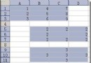
用上面的代碼結合這個截圖，如果從A1單元格開始進行數據篩選，如果Field的值為1，則表示取列表中的第一個字段即B列，以此類推，如果Field的值為2則表示C列…不過前提是所有的待篩選列表是連續的，就是說中間不能有空列。當然也可以這樣，使用Range(“A1:E17”).AutoFilter，這樣即使待篩選列表中有空列也可以，因為已經指定了一個待篩選區域。Field的值表示的就是將篩選條件應用到所表示的列上。下面是一些使用AutoFilter的例子。

Sub SimpleOrFilter()
Worksheets("SalesReport").Select
Range("A1").AutoFilter
Range("A1").AutoFilter Field:=4,Criteria1:="=A", Operator:=xlOr, Criteria2:="=B"
End Sub

Sub SimpleAndFilter()
Worksheets("SalesReport").Select
Range("A1").AutoFilter
Range("A1").AutoFilter Field:=4, _
Criteria1:=">=A", _
Operator:=xlAnd, Criteria2:="<=EZZ"
End Sub

Sub Top10Filter()
' Top 12 Revenue Records
Worksheets("SalesReport").Select
Range("A1").AutoFilter
Range("A1").AutoFilter Field:=6, Criteria1:="12",Operator:=xlTop10Items
End Sub

Sub MultiSelectFilter()
Worksheets("SalesReport").Select
Range("A1").AutoFilter
Range("A1").AutoFilter Field:=4, Criteria1:=Array("A", "C", "E","F", "H"),Operator:=xlFilterValues
End Sub

Sub DynamicAutoFilter()
Worksheets("SalesReport").Select
Range("A1").AutoFilter
Range("A1").AutoFilter Field:=3,Criteria1:=xlFilterNextYear,Operator:=xlFilterDynamic
End Sub

Sub FilterByIcon()
Worksheets("SalesReport").Select
Range("A1").AutoFilter
Range("A1").AutoFilter Field:=6, _
Criteria1:=ActiveWorkbook.IconSets(xl5ArrowsGray).Item(5),Operator:=xlFilterIcon
End Sub

Sub FilterByFillColor()
Worksheets("SalesReport").Select
Range("A1").AutoFilter
Range("A1").AutoFilter Field:=6, Criteria1:=RGB(255, 0, 0), Operator:=xlFilterCellColor
End Sub

下面的程序是通過Excel的AutoFilter功能快速刪除行的方法，供參考：

Sub DeleteRows3()
Dim lLastRow As　Long　　　　　　 'Last row
Dim rng As range
Dim rngDelete As range
'Freeze screen
Application.ScreenUpdating =　False
'Insert dummy row for dummy field name
Rows(1).Insert
'Insert dummy field name
range("C1").value =　"Temp"
With ActiveSheet
.UsedRange
lLastRow = .cells.SpecialCells(xlCellTypeLastCell).row
Set rng = range("C1", cells(lLastRow, "C"))
rng.AutoFilter Field:=1, Criteria1:="Mangoes"
Set rngDelete = rng.SpecialCells(xlCellTypeVisible)
rng.AutoFilter
rngDelete.EntireRow.delete
.UsedRange
End　With
End Sub

Binding

1.一個使用早期Binging的例子

Sub EarlyBinding()
Dim objExcel As Excel.Application
Set objExcel =　New Excel.Application
With objExcel
.Visible =　True
.Workbooks.Add
.Range("A1") =　"Hello World"
End　With
End Sub

2.使用CreateObject創建Excel實例

Sub LateBinding()

'Declare a generic object variable
Dim objExcel As　Object

'Point the object variable at an Excel application object
Set objExcel =　CreateObject("Excel.Application")

'Set properties and execute methods of the object
With objExcel
.Visible =　True
.Workbooks.Add
.Range("A1") =　"Hello World"
End　With

End Sub

3.使用CreateObject創建指定版本的Excel實例

Sub mate()
Dim objExcel As　Object

Set objExcel =　CreateObject("Excel.Application.8")
End Sub

當Create對象實例之後，就可以使用該對象的所有屬性和方法了，如SaveAs方法、Open方法、Application屬性等。

Cell Comments

1.獲取單元格的備注

Private　Sub CommandButton1_Click()
Dim strGotIt As　String
strGotIt = WorksheetFunction.Clean(Range("A1").Comment.Text)
MsgBox strGotIt
End Sub

Range.Comment.Text用於得到單元格的備注文本，如果當前單元格沒有添加備注，則會引發異常。注意代碼中使用了WorksheetFunction對象，該對象是Excel的系統對象，它提供了很多系統函數，這裡用到的Clean函數用於清楚指定文本中的所有關鍵字（特殊字符），具體信息可以查閱Excel自帶的幫助文檔，裡面提供的函數非常多。下面是一個使用Application.WorksheetFunction.Substitute函數的例子，其中第一個Substitute將給定的字符串中的author:替換為空字符串，第二個Substitute將給定的字符串中的空格替換為空字符串。

Private　Function CleanComment(author As　String, cmt As　String) As　String
Dim tmp As　String

tmp = Application.WorksheetFunction.Substitute(cmt, author &　":", "")
tmp = Application.WorksheetFunction.Substitute(tmp, Chr(10), "")

CleanComment = tmp
End Function

2.修改Excel單元格內容時自動給單元格添加Comments信息

Private　Sub Worksheet_Change(ByVal Target As Excel.Range)
Dim newText As　String
Dim oldText As　String

For　Each cell In Target
With cell
On　Error　Resume　Next
oldText = .Comment.Text
If Err <>　0　Then .AddComment
newText = oldText &　" Changed by "　& Application.UserName &　" at "　&　Now　& vbLf
MsgBox newText
.Comment.Text newText
.Comment.Visible =　True
.Comment.Shape.Select
Selection.AutoSize =　True
.Comment.Visible =　False
End　With
Next cell
End Sub

Comments內容可以根據需要自己修改，Worksheet_Change方法在Worksheet單元格內容被修改時執行。

3.改變Comment標簽的顯示狀態

Sub ToggleComments()
If Application.DisplayCommentIndicator = xlCommentAndIndicator Then
Application.DisplayCommentIndicator = xlCommentIndicatorOnly
Else
Application.DisplayCommentIndicator = xlCommentAndIndicator
End　If
End Sub

Application.DisplayCommentIndicator有三種狀態：xlCommentAndIndicator-始終顯示Comment標簽、xlCommentIndicatorOnly-當鼠標指向單元格的Comment pointer時顯示Comment標簽、xlNoIndicator-隱藏Comment標簽和單元格的Comment pointer。

4.改變Comment標簽的默認大小

Sub CommentFitter1()
With Range("A1").Comment
.Shape.Width =　150
.Shape.Height =　300
End　With
End Sub

注意：舊版本中的Range.NoteText方法同樣可以返回單元格中的Comment，按照Excel的幫助文檔中的介紹，建議在新版本中統一使用Range.Comment方法。

Cell Copy

1.從一個Sheet中的Range拷貝數據到另一個Sheet中的Range

Private　Sub CommandButton1_Click()
Dim myWorksheet As Worksheet
Dim myWorksheetName As　String

myWorksheetName =　"MyName"
Sheets.Add.Name = myWorksheetName
Sheets(myWorksheetName).Move After:=Sheets(Sheets.Count)
Sheets("Sheet1").Range("A1:A5").Copy Sheets(myWorksheetName).Range("A1")
End Sub

Sheets.Add.Name = myWorksheetName用於在Sheets集合中添加名稱為myWorksheetName的Sheet，Sheets(myWorksheetName).Move After:=Sheets(Sheets.Count)將剛剛添加的這個Sheet移到Sheets集合中最後一個元素的後面，最後Range.Copy方法將數據拷貝到新表中對應的單元格中。

Cell Format

1.設置單元格文字的顏色

Sub fontColor()
Cells.Font.Color = vbRed
End Sub

Color的值可以通過RGB(0,225,0)這種方式獲取，也可以使用Color常數： 常數 值 描述 vbBlack 0x0 黑色 vbRed 0xFF 紅色 vbGreen 0xFF00 綠色 vbYellow 0xFFFF 黃色 vbBlue 0xFF0000 藍色 vbMagenta 0xFF00FF 紫紅色 vbCyan 0xFFFF00 青色 vbWhite 0xFFFFFF 白色

2.通過ColorIndex屬性修改單元格字體的顏色

通過上面的方法外，還可以通過指定Range.Font.ColorIndex屬性來修改單元格字體的顏色，該屬性表示了調色板中顏色的索引值，也可以指定一個常量，xlColorIndexAutomatic（-4105）為自動配色，xlColorIndexNone（-4142）表示無色。

3.一個Format單元格的例子

Sub cmd()
Cells(1, "D").Value =　"Text"
Cells(1, "D").Select

With Selection
.Font.Bold =　True
.Font.Name =　"Arial"
.Font.Size =　72
.Font.Color =　RGB(0, 0, 255)　 'Dark blue
.Columns.AutoFit
.Interior.Color =　RGB(0, 255, 255) 'Cyan
.Borders.Weight = xlThick
.Borders.Color =　RGB(0, 0, 255)　 'Dark Blue
End　With
End Sub

4.指定單元格的邊框樣式

Sub UpdateBorder
range("A1").Borders(xlRight).LineStyle = xlLineStyleNone
range("A1").Borders(xlLeft).LineStyle = xlContinuous
range("A1").Borders(xlBottom).LineStyle = xlDashDot
range("A1").Borders(xlTop).LineStyle = xlDashDotDot　　　　
End Sub

如果要為Range的四個邊框設置同樣的樣式，可以直接設置Range.Borders.LineStyle的值，該值為一個常數： 名稱 值 描述 xlContinuous 1 實線 xlDash -4115 虛線 xlDashDot 4 點劃相間線 xlDashDotDot 5 劃線後跟兩個點 xlDot -4118 點式線 xlDouble -4119 雙線 xlLineStyleNone -4142 無線 xlSlantDashDot 13 傾斜的劃線

Cell Number Format

改變單元格數值的格式

Sub FormatCell()
Dim myVar As Range
Set myVar = Selection
With myVar
.NumberFormat =　"#,##0.00_);[Red](#,##0.00)"
.Columns.AutoFit
End　With

End Sub

單元格數值的格式有很多種，如數值、貨幣、日期等，具體的格式指定樣式可以通過錄制Excel宏得知，在Excel的Sheet中選中一個單元格，然後單擊右鍵，選擇“設置單元格格式”，在“數字”選項卡中進行選擇。

Cell Value

1.使用STRConv函數轉換Cell中的Value值

Sub STRConvDemo()
Cells(3, "A").Value = STRConv("ALL LOWERCASE ", vbLowerCase)
End Sub

STRConv是一個功能很強的系統函數，它可以按照指定的轉換類型轉換字符串值，如大小寫轉換、將字符串中的首字母大寫、單雙字節字符轉換、平假名片假名轉換、Unicode字符集轉換等。具體的使用規則和參數類型讀者可以查閱一下Excel自帶的幫助文檔，在幫助中輸入STRConv，查看搜索結果中的第一項。

2.使用Format函數進行字符串的大小寫轉換

Sub callLower()
Cells(2, "A").Value = Format("ALL LOWERCASE ", "<")
End Sub

Format也是一個非常常用的系統函數，它用於格式化輸出字符串，有關Format的使用讀者可以查看Excel自帶的幫助文檔。Format函數有很多的使用技巧，如本例給出的<可以將字符串轉換為小寫形式，相應地，>則可以將字符串轉換為大寫形式。

3.一種引用單元格的快捷方法

Sub GetSum()　　　　　　　　　　　　　　　　　　　 ' using the shortcut approach
[A1].Value = Application.Sum([E1:E15])
End Sub

[A1]即等效於Range("A1")，這是一種引用單元格的快捷方法，在公式中同樣也可以使用。

4.計算單元格中的公式

Sub CalcCell()
Worksheets("Sheet1").range("A1").Calculate
End Sub

示例中的代碼將計算Sheet1工作表中A1單元格的公式，相應地，Application.Calculate可以計算所有打開的工作簿中的公式。

5.一個用於檢查單元格數據類型的例子

Function CellType(Rng)
Application.Volatile
Set Rng = Rng.Range("A1")
Select　Case　True
Case　IsEmpty(Rng)
CellType =　"Blank"
Case WorksheetFunction.IsText(Rng)
CellType =　"Text"
Case WorksheetFunction.IsLogical(Rng)
CellType =　"Logical"
Case WorksheetFunction.IsErr(Rng)
CellType =　"Error"
Case　IsDate(Rng)
CellType =　"Date"
Case　InStr(1, Rng.Text, ":") <>　0
CellType =　"Time"
Case　IsNumeric(Rng)
CellType =　"Value"
End　Select
End Function

Application.Volatile用於將用戶自定義函數標記為易失性函數，有關該方法的具體應用，讀者可以查閱Excel自帶的幫助文檔。

6.一個Excel單元格行列變換的例子

Public　Sub Transpose()
Dim I As　Integer
Dim J As　Integer
Dim transArray(9, 2) As　Integer
For I =　1　To　3
For J =　1　To　10
transArray(J -　1, I -　1) = Cells(J, Chr(I +　64)).Value
Next J
Next I
Range("A1:C10").ClearContents
For I =　1　To　3
For J =　1　To　10
Cells(I, Chr(J +　64)).Value = transArray(J -　1, I -　1)
Next J
Next I
End Sub

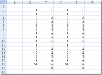
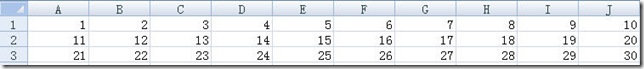
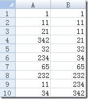
該示例將A1:C10矩陣中的數據進行行列轉換。

轉換前：

轉換後：

7.VBA中冒泡排序示例

Public　Sub BubbleSort2()
Dim tempVar As　Integer
Dim anotherIteration As　Boolean
Dim I As　Integer
Dim myArray(10) As　Integer
For I =　1　To　10
myArray(I -　1) = Cells(I, "A").Value
Next I
Do
anotherIteration =　False
For I =　0　To　8
If myArray(I) > myArray(I +　1) Then
tempVar = myArray(I)
myArray(I) = myArray(I +　1)
myArray(I +　1) = tempVar
anotherIteration =　True
End　If
Next I
Loop　While anotherIteration =　True
For I =　1　To　10
Cells(I, "B").Value = myArray(I -　1)
Next I
End Sub

該實例將A1:A10中的數值按從小到大的順序進行並，並輸出到B1:B10的單元格中。

8.一個驗證Excel單元格數據輸入規范的例子

Private　Sub Worksheet_Change(ByVal Target As Range)
Dim cellContents As　String
Dim valLength As　Integer
cellContents =　Trim(Str(Val(Target.Value)))
valLength =　Len(cellContents)
If valLength <>　3　Then
MsgBox ("Please enter a 3 digit area code.")
Cells(9, "C").Select
Else
Cells(9, "C").Value = cellContents
Cells(9, "D").Select
End　If
End Sub

重點看一下Val函數，該函數返回給定的字符串中的數字，數字之外的字符將被忽略掉，該示例用於檢測用戶單元格的輸入值，如果輸入值中包含的數字個數不等於3，則提示用戶，否則就將其中的數字賦值給另一個單元格。

Cell

1.查找最後一個單元格

Sub　GetLastCell()
Dim　RealLastRow　As　Long
Dim　RealLastColumn　As　Long

Range("A1").Select
On　Error　Resume　Next
RealLastRow　=　Cells.Find("*",　Range("A1"),　xlFormulas,　,　xlByRows,　xlPrevious).Row
RealLastColumn　=　Cells.Find("*",　Range("A1"),　xlFormulas,　,　xlByColumns,　xlPrevious).Column
Cells(RealLastRow,　RealLastColumn).Select
End　Sub

該示例用來查找出當前工作表中的最後單元，並將其選中，主要使用了Cells對象的Find方法，有關該方法的詳細說明讀者可以參考Excel自帶的幫助文檔，搜索Cells.Find，見Range.Find方法的說明。

2.判斷一個單元格是否為空

Sub　ShadeEveryRowWithNotEmpty()
Dim　i　As　Integer
i　=　1
Do　Until　IsEmpty(Cells(i,　1))
Cells(i,　1).EntireRow.Interior.ColorIndex　=　15
i　=　i　+　1
Loop
End　Sub

IsEmpty函數本是用來判斷變量是否已經初始化的，它也可以被用來判斷單元格是否為空，該示例從A1單元格開始向下檢查單元格，將其所在行的背景色設置成灰色，直到下一個單元格的內容為空。

3.判斷當前單元格是否為空的另外一種方法

Sub　IsActiveCellEmpty()
Dim　sFunctionName　As　String,　sCellReference　As　String
sFunctionName　=　"ISBLANK"
sCellReference　=　ActiveCell.Address
MsgBox　Evaluate(sFunctionName　&　"("　&　sCellReference　&　")")
End　Sub

Evaluate方法用來計算給定的表達式，如計算一個公式Evaluate("Sin(45)")，該示例使用Evaluate方法計算ISBLANK表達式，該表達式用來判斷指定的單元格是否為空，如Evaluate(ISBLANK(A1))。

4.一個在給定的區域中找出數值最大的單元格的例子

Sub　GoToMax()
Dim　WorkRange　As　range

If　TypeName(Selection)　<>　"Range"　Then　Exit　Sub

If　Selection.Count　=　1　Then
Set　WorkRange　=　Cells
Else
Set　WorkRange　=　Selection
End　If
MaxVal　=　Application.Max(WorkRange)
On　Error　Resume　Next
WorkRange.Find(What:=MaxVal,　_
After:=WorkRange.range("A1"),　_
LookIn:=xlValues,　_
LookAt:=xlPart,　_
SearchOrder:=xlByRows,　_
SearchDirection:=xlNext,　MatchCase:=False　_
).Select
If　Err　<>　0　Then　MsgBox　"Max　value　was　not　found:　"　_
&　MaxVal
End　Sub

5.使用數組更快地填充單元格區域

Sub　ArrayFillRange()
Dim　TempArray()　As　Integer
Dim　TheRange　As　range

CellsDown　=　3
CellsAcross　=　4
StartTime　=　timer

ReDim　TempArray(1　To　CellsDown,　1　To　CellsAcross)
Set　TheRange　=　ActiveCell.range(Cells(1,　1),　Cells(CellsDown,　CellsAcross))
CurrVal　=　0
Application.ScreenUpdating　=　False
For　I　=　1　To　CellsDown
For　J　=　1　To　CellsAcross
TempArray(I,　J)　=　CurrVal　+　1
CurrVal　=　CurrVal　+　1
Next　J
Next　I

TheRange.value　=　TempArray
Application.ScreenUpdating　=　True
MsgBox　Format(timer　-　StartTime,　"00.00")　&　"　seconds"
End　Sub

該示例展示了將一個二維數組直接賦值給一個“等效”單元格區域的方法，利用該方法可以使用數組直接填充單元格區域，結合下面這個直接在循環中填充單元格區域的方法，讀者可以自己驗證兩種方法在效率上的差別。

Sub　LoopFillRange()
Dim　CurrRow　As　Long,　CurrCol　As　Integer
Dim　CurrVal　As　Long

CellsDown　=　3
CellsAcross　=　4
StartTime　=　timer
CurrVal　=　1
Application.ScreenUpdating　=　False
For　CurrRow　=　1　To　CellsDown
For　CurrCol　=　1　To　CellsAcross
ActiveCell.Offset(CurrRow　-　1,　_
CurrCol　-　1).value　=　CurrVal
CurrVal　=　CurrVal　+　1
Next　CurrCol
Next　CurrRow

'　　　Display　elapsed　time
Application.ScreenUpdating　=　True
MsgBox　Format(timer　-　StartTime,　"00.00")　&　"　seconds"
End　Sub