數據源是科比籃球比賽的一個數據集
我們先簡單的看一下數據集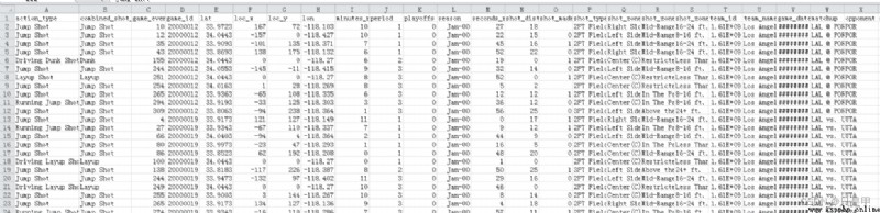
特征值簡介:action_type 進攻方式(更具體)combined_shot_type 進攻方式game_event_id 比賽時間idgame_id 比賽IDlat 投籃點loc_x 投籃點loc_y 投籃點lon 投籃點minutes_remaining 單節剩余時間(分鐘)period 表示第幾節playoffs 是否是季後賽season 賽季seconds_remaining 剩余時間(秒)shot_distance 投籃距離shot_made_flag 是否進球shot_type 兩分球或三分球shot_zone_area 投籃區域shot_zone_basic 投籃區域(更具體)shot_zone_range 投籃范圍team_id 球隊IDteam_name 球隊名稱game_date 比賽日期matchup 比賽雙方opponent 對手shot_id 投籃ID
代碼:
import numpy as np
import pandas as pd
import matplotlib.pyplot as plt
from sklearn.ensemble import RandomForestClassifier
from sklearn.model_selection import KFold
# 讀取數據源
filename = "E:/file/data.csv"
raw = pd.read_csv(filename)
#print(raw.head(10))
# 選擇標簽值不為null的
kobe = raw[pd.notnull(raw['shot_made_flag'])]
# 畫圖
alpha = 0.02
plt.figure(figsize=(10, 10))
# x軸和y軸
plt.subplot(121)
plt.scatter(kobe.loc_x, kobe.loc_y, color='r', alpha=alpha)
plt.title('loc_x and loc_y')
# 精度和維度
plt.subplot(122)
plt.scatter(kobe.lon, kobe.lat, color='b', alpha=alpha)
plt.title('lat and lon')
plt.show()
測試記錄:
從圖中我們可以看到,loc_x和loc_y 以及 lat和lon 這些都代表了坐標,可看到kobe投籃位置的分布。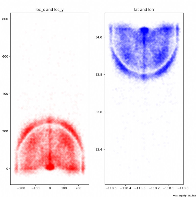
通過我們簡單的分析可以看到數據集存在如下問題:
shot_made_flag 這個標簽值有缺失值loc_x 有為0的異常值season 特征值格式混亂做數據預處理的時候,我們需要解決上述問題
代碼:
import numpy as np
import pandas as pd
import matplotlib.pyplot as plt
from sklearn.ensemble import RandomForestClassifier
from sklearn.model_selection import KFold
# 讀取數據源
filename = "E:/file/data.csv"
raw = pd.read_csv(filename)
#print(raw.head(10))
# 選擇標簽值不為null的
kobe = raw[pd.notnull(raw['shot_made_flag'])]
# 根據X軸和Y軸來計算距離,衍生一個特征
raw['dist'] = np.sqrt(raw['loc_x']**2 + raw['loc_y']**2)
# 處理loc_x 為0的異常數據
loc_x_zero = raw['loc_x'] == 0
#print (loc_x_zero)
raw['angle'] = np.array([0]*len(raw))
raw['angle'][~loc_x_zero] = np.arctan(raw['loc_y'][~loc_x_zero] / raw['loc_x'][~loc_x_zero])
raw['angle'][loc_x_zero] = np.pi / 2
# 將比賽剩余的分鐘和秒 加起來,衍生一個特征
raw['remaining_time'] = raw['minutes_remaining'] * 60 + raw['seconds_remaining']
# 查看特征的唯一值
print("查看特征的唯一值")
print(kobe.action_type.unique())
print(kobe.combined_shot_type.unique())
print(kobe.shot_type.unique())
print(kobe.shot_type.value_counts())
print("處理season格式不統一的問題")
kobe['season'].unique()
raw['season'] = raw['season'].apply(lambda x: int(x.split('-')[1]))
print(raw['season'].unique())
測試記錄:
查看特征的唯一值
['Jump Shot' 'Driving Dunk Shot' 'Layup Shot' 'Running Jump Shot'
'Reverse Dunk Shot' 'Slam Dunk Shot' 'Driving Layup Shot'
'Turnaround Jump Shot' 'Reverse Layup Shot' 'Tip Shot'
'Running Hook Shot' 'Alley Oop Dunk Shot' 'Dunk Shot'
'Alley Oop Layup shot' 'Running Dunk Shot' 'Driving Finger Roll Shot'
'Running Layup Shot' 'Finger Roll Shot' 'Fadeaway Jump Shot'
'Follow Up Dunk Shot' 'Hook Shot' 'Turnaround Hook Shot' 'Jump Hook Shot'
'Running Finger Roll Shot' 'Jump Bank Shot' 'Turnaround Finger Roll Shot'
'Hook Bank Shot' 'Driving Hook Shot' 'Running Tip Shot'
'Running Reverse Layup Shot' 'Driving Finger Roll Layup Shot'
'Fadeaway Bank shot' 'Pullup Jump shot' 'Finger Roll Layup Shot'
'Turnaround Fadeaway shot' 'Driving Reverse Layup Shot'
'Driving Slam Dunk Shot' 'Step Back Jump shot' 'Turnaround Bank shot'
'Reverse Slam Dunk Shot' 'Floating Jump shot' 'Putback Slam Dunk Shot'
'Running Bank shot' 'Driving Bank shot' 'Driving Jump shot'
'Putback Layup Shot' 'Putback Dunk Shot' 'Running Finger Roll Layup Shot'
'Pullup Bank shot' 'Running Slam Dunk Shot' 'Cutting Layup Shot'
'Driving Floating Jump Shot' 'Running Pull-Up Jump Shot' 'Tip Layup Shot'
'Driving Floating Bank Jump Shot']
['Jump Shot' 'Dunk' 'Layup' 'Tip Shot' 'Hook Shot' 'Bank Shot']
['2PT Field Goal' '3PT Field Goal']
2PT Field Goal 20285
3PT Field Goal 5412
Name: shot_type, dtype: int64
處理season格式不統一的問題
[ 1 2 3 4 5 6 7 8 9 10 11 12 13 14 15 16 97 98 99 0]
如果特征值之間存在線性關系,此時我們只需要使用其中之一即可,無需使用多個特征值。
代碼:
import numpy as np
import pandas as pd
import matplotlib.pyplot as plt
from sklearn.ensemble import RandomForestClassifier
from sklearn.model_selection import KFold
# 讀取數據源
filename = "E:/file/data.csv"
raw = pd.read_csv(filename)
#print(raw.head(10))
# 根據X軸和Y軸來計算距離,衍生一個特征
raw['dist'] = np.sqrt(raw['loc_x']**2 + raw['loc_y']**2)
# 畫散點圖
# 這個兩個特征值呈線性關系,用一個即可
plt.figure(figsize=(5, 5))
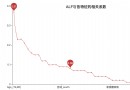
plt.scatter(raw['dist'], raw['shot_distance'], color='blue')
plt.title('dist and shot_distance')
plt.show()
測試記錄:
從圖中我們可以看到,這兩個特征值完全呈線性關系,此時我們只需要使用一個特征值即可。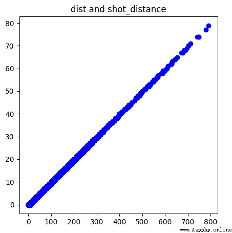
代碼:
import numpy as np
import pandas as pd
import matplotlib.pyplot as plt
from sklearn.ensemble import RandomForestClassifier
from sklearn.model_selection import KFold
# 讀取數據源
filename = "E:/file/data.csv"
raw = pd.read_csv(filename)
#print(raw.head(10))
# 選擇標簽值不為null的
kobe = raw[pd.notnull(raw['shot_made_flag'])]
# 聚合查看數據
gs = kobe.groupby('shot_zone_area')
print(kobe['shot_zone_area'].value_counts())
print (len(gs))
測試記錄:
Center(C) 11289
Right Side Center(RC) 3981
Right Side(R) 3859
Left Side Center(LC) 3364
Left Side(L) 3132
Back Court(BC) 72
Name: shot_zone_area, dtype: int64
6
代碼:
import numpy as np
import pandas as pd
import matplotlib.pyplot as plt
from sklearn.ensemble import RandomForestClassifier
from sklearn.model_selection import KFold
import matplotlib.cm as cm
# 讀取數據源
filename = "E:/file/data.csv"
raw = pd.read_csv(filename)
#print(raw.head(10))
# 處理loc_x 為0的異常數據
loc_x_zero = raw['loc_x'] == 0
#print (loc_x_zero)
raw['angle'] = np.array([0]*len(raw))
raw['angle'][~loc_x_zero] = np.arctan(raw['loc_y'][~loc_x_zero] / raw['loc_x'][~loc_x_zero])
raw['angle'][loc_x_zero] = np.pi / 2
# 將比賽剩余的分鐘和秒 加起來,衍生一個特征
raw['remaining_time'] = raw['minutes_remaining'] * 60 + raw['seconds_remaining']
# 選擇標簽值不為null的
kobe = raw[pd.notnull(raw['shot_made_flag'])]
# 畫圖
plt.figure(figsize=(20, 10))
def scatter_plot_by_category(feat):
alpha = 0.1
gs = kobe.groupby(feat)
cs = cm.rainbow(np.linspace(0, 1, len(gs)))
for g, c in zip(gs, cs):
plt.scatter(g[1].loc_x, g[1].loc_y, color=c, alpha=alpha)
# shot_zone_area
plt.subplot(131)
scatter_plot_by_category('shot_zone_area')
plt.title('shot_zone_area')
# shot_zone_basic
plt.subplot(132)
scatter_plot_by_category('shot_zone_basic')
plt.title('shot_zone_basic')
# shot_zone_range
plt.subplot(133)
scatter_plot_by_category('shot_zone_range')
plt.title('shot_zone_range')
plt.show()
測試記錄: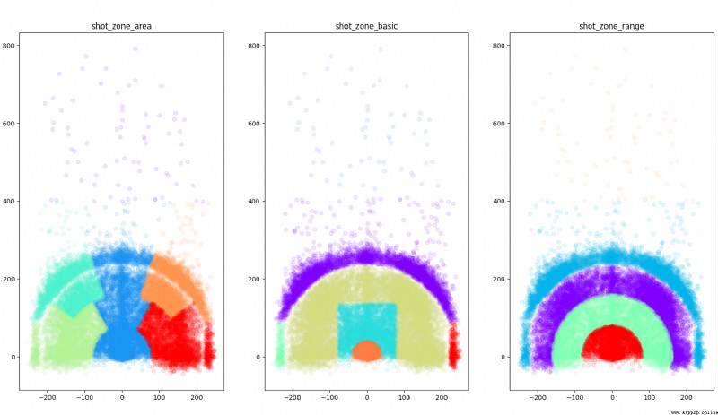
在對變量進行獨熱編碼時使用,例如:某一列類別型變量是季節,取值為春、夏、秋、冬,當我們對其進行建模時,需要將其進行獨熱編碼,這時:pandas.get_dummies便派上了用場。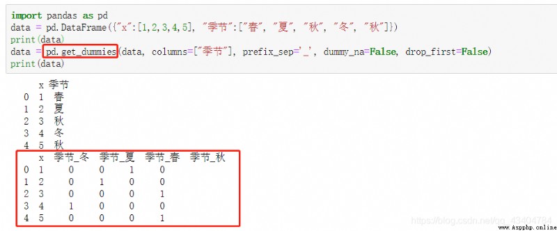
data : array-like, Series, or DataFrame 輸入的數據prefix : string, get_dummies轉換後,列名的前綴,默認為Nonecolumns : 指定需要實現類別轉換的列名 否則轉換所有類別性的列dummy_na : bool, default False 增加一列表示空缺值,如果False就忽略空缺值drop_first : bool, default False 獲得k中的k-1個類別值,去除第一個,防止出現多重共線性
代碼:
import numpy as np
import pandas as pd
import matplotlib.pyplot as plt
from sklearn.ensemble import RandomForestClassifier
from sklearn.model_selection import StratifiedKFold
import matplotlib.cm as cm
from sklearn.ensemble import RandomForestRegressor
from sklearn.metrics import confusion_matrix, log_loss
import time
# 讀取數據源
filename = "E:/file/data.csv"
raw = pd.read_csv(filename)
#print(raw.head(10))
# 將不需要的特征值進行刪除
drops = ['shot_id', 'team_id', 'team_name', 'shot_zone_area', 'shot_zone_range', 'shot_zone_basic', \
'matchup', 'lon', 'lat', 'seconds_remaining', 'minutes_remaining', \
'shot_distance', 'loc_x', 'loc_y', 'game_event_id', 'game_id', 'game_date']
for drop in drops:
raw = raw.drop(drop, 1)
#print(raw['combined_shot_type'].value_counts())
#pd.get_dummies(raw['combined_shot_type'], prefix='combined_shot_type')[0:2]
categorical_vars = ['action_type', 'combined_shot_type', 'shot_type', 'opponent', 'period', 'season']
for var in categorical_vars:
raw = pd.concat([raw, pd.get_dummies(raw[var], prefix=var)], 1)
raw = raw.drop(var, 1)
# 劃分訓練集和測試集
train_kobe = raw[pd.notnull(raw['shot_made_flag'])]
train_label = train_kobe['shot_made_flag'].astype(np.int64)
train_kobe = train_kobe.drop('shot_made_flag', 1)
test_kobe = raw[pd.isnull(raw['shot_made_flag'])]
test_kobe = test_kobe.drop('shot_made_flag', 1)
print('Finding best n_estimators for RandomForestClassifier...')
min_score = 100000
best_n = 0
scores_n = []
range_n = np.logspace(0, 2, num=3, dtype=np.int64).astype(np.int64)
for n in range_n:
print("the number of trees : {0}".format(n))
t1 = time.time()
rfc_score = 0.
rfc = RandomForestClassifier(n_estimators=n)
skfolds = StratifiedKFold(
n_splits=3,
random_state=42, # 設置隨機種子
shuffle=True
)
for train_k, test_k in skfolds.split(train_kobe, train_label):
rfc.fit(train_kobe.iloc[train_k], train_label.iloc[train_k])
# rfc_score += rfc.score(train.iloc[test_k], train_y.iloc[test_k])/10
pred = rfc.predict(train_kobe.iloc[test_k])
rfc_score += log_loss(train_label.iloc[test_k], pred) / 10
scores_n.append(rfc_score)
if rfc_score < min_score:
min_score = rfc_score
best_n = n
t2 = time.time()
print('Done processing {0} trees ({1:.3f}sec)'.format(n, t2 - t1))
print(best_n, min_score)
# find best max_depth for RandomForestClassifier
print('Finding best max_depth for RandomForestClassifier...')
min_score = 100000
best_m = 0
scores_m = []
range_m = np.logspace(0, 2, num=3, dtype=np.int64).astype(np.int64)
for m in range_m:
print("the max depth : {0}".format(m))
t1 = time.time()
skfolds = StratifiedKFold(
n_splits=3,
random_state=42, # 設置隨機種子
shuffle=True
)
rfc_score = 0.
rfc = RandomForestClassifier(max_depth=m, n_estimators=best_n)
for train_k, test_k in skfolds.split(train_kobe, train_label):
rfc.fit(train_kobe.iloc[train_k], train_label.iloc[train_k])
# rfc_score += rfc.score(train.iloc[test_k], train_y.iloc[test_k])/10
pred = rfc.predict(train_kobe.iloc[test_k])
rfc_score += log_loss(train_label.iloc[test_k], pred) / 10
scores_m.append(rfc_score)
if rfc_score < min_score:
min_score = rfc_score
best_m = m
t2 = time.time()
print('Done processing {0} trees ({1:.3f}sec)'.format(m, t2 - t1))
print(best_m, min_score)
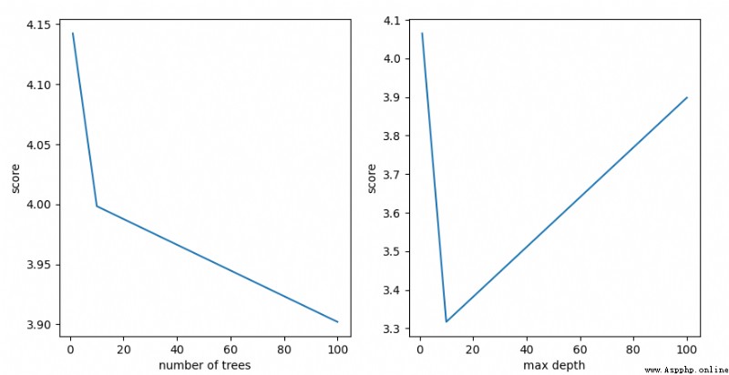
plt.figure(figsize=(10, 5))
plt.subplot(121)
plt.plot(range_n, scores_n)
plt.ylabel('score')
plt.xlabel('number of trees')
plt.subplot(122)
plt.plot(range_m, scores_m)
plt.ylabel('score')
plt.xlabel('max depth')
plt.show()
測試記錄:
Finding best n_estimators for RandomForestClassifier...
the number of trees : 1
Done processing 1 trees (0.556sec)
the number of trees : 10
Done processing 10 trees (1.138sec)
the number of trees : 100
Done processing 100 trees (10.486sec)
100 3.9020328477633024
Finding best max_depth for RandomForestClassifier...
the max depth : 1
Done processing 1 trees (1.294sec)
the max depth : 10
Done processing 10 trees (3.215sec)
the max depth : 100
Done processing 100 trees (10.556sec)
10 3.316936324282448