The stock market is vulnerable to many uncertain factors , Therefore, the challenge of stock price prediction is huge , It has been a hot research field in digital finance since it was proposed . Traditional simple K Line 、 The operation of crosshair method is simple , But the prediction accuracy is not satisfactory . With the deepening of this research field , Various modeling methods emerge in endlessly . To compare the performance of various models , This paper selects four representative models , Moving average in linear model 、 Linear regression , Traditional machine learning model KNN, Deep learning model LSTM, Four models are used to fit and predict the stock price of Shenzhen Ping An Bank . Comprehensive comparison found that , Deep network has its unique advantages in high noise 、 High volatility 、 Excellent performance in non-linear financial time series data , Deep learning provides new ideas for stock price prediction . Finally, this article uses LSTM Model for the future of Ping An Bank 30 Predict the stock price trend in a working day and put forward relevant suggestions to investors .
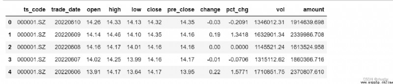
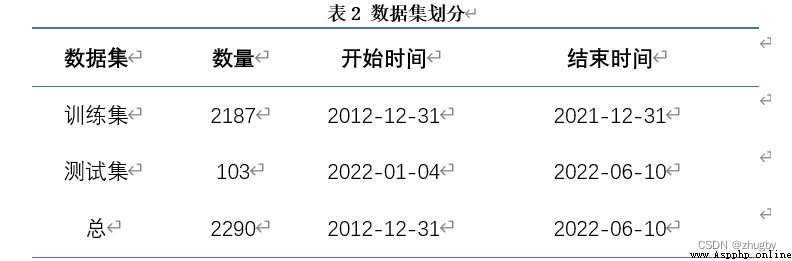
The data set used in this article is 2012 year 12 month 31 solstice 2022 year 6 month 10 The daily historical market data of Shenzhen Stock Exchange Ping An Bank , common 2290 strip . By calling the data interface from tushare pro Get... On the platform ,tushare It's a python Financial data interface package , Currently, open source is free , Help data analysts reduce a lot of pressure on data acquisition . Mainly by Shanghai Stock Exchange 、 The shenzhen stock exchange 、 Tencent Finance 、 Sina 、 Phoenix finance, etc tushare Some data on stocks and securities provided , This includes historical data 、 real-time data 、 Classified data 、 Fundamental data 、 Macroeconomic data 、 Internet public opinion 、 News event data and so on , It provides a good tool for data analysis of financial market and development of financial products . The data of this article is provided by Shenzhen Stock Exchange , True and reliable . There are stock codes in the data set (ts_code)、 Transaction date (trade_date)、 Opening price (open)、 Highest price (high)、 The lowest price (low)、 Closing price (close)、 Prec (pre_close)、 Up and down (change) etc. 11 Two variables . As shown in Figure 1 :

The work of data preprocessing in this paper mainly includes checking whether there are missing values in the data , Convert a character date to Datatime Date type . Because the data set is relatively clean , A lot of pretreatment work is reduced .
import tushare as ts
token='******' # Write your own here api Interface token
pro = ts.pro_api(token)
# Ping An Bank stock data download
df = pro.daily(ts_code='000001.SZ', start_date='20121231', end_date='20220612')
df.to_csv(' Historical quotation of Ping An Bank 1.csv')
#import packages
import pandas as pd
import numpy as np
#to plot within notebook
import matplotlib.pyplot as plt
%matplotlib inline
#setting figure size
from matplotlib.pylab import rcParams
rcParams['figure.figsize'] = 20,10
#for normalizing data
from sklearn.preprocessing import MinMaxScaler
scaler = MinMaxScaler(feature_range=(0, 1))
#read the file
df = pd.read_csv(' Historical quotation of Ping An Bank 1.csv',index_col=0)
#print the head
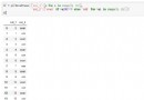
df.head()otput:
# The definition will int Type date to dataframe type
def string_to_date(string: str) -> str:
""" String to date format """
from datetime import datetime
shift_datetime = datetime.strptime(string, '%Y%m%d') # character string -> Time
shift_date = shift_datetime.strftime("%Y-%m-%d") # Time -> Arbitrary time format
return shift_date
def convert_date_from_int(time_series: pd.Series):
""" Plastic series -> pandas Time format """
time_series = time_series.astype('str').apply(string_to_date)
return pd.to_datetime(time_series)
output:
Simply analyze the significance of each variable , The invoiced price and closing price of the stock represent the starting price and final price of the stock on a certain day ; Highest price 、 The lowest price means the highest and lowest price of a stock transaction on a certain day ; The amount of rise and fall and rise and fall are the amount and range of change of the closing price of the stock compared with the previous day ; Trading volume represents the total number of stocks traded on that day ; The turnover represents the turnover of a company on that day . What is recorded in the data is the stock trading data on weekdays , Therefore, there will be some missing dates , No additional filling treatment is required , After processing, it will affect the prediction results . Generally speaking , The gains and losses of stocks are determined by the closing price , Therefore, the target variable of stock prediction is the closing price . We are analyzing financial time series data , So the independent variable is time .
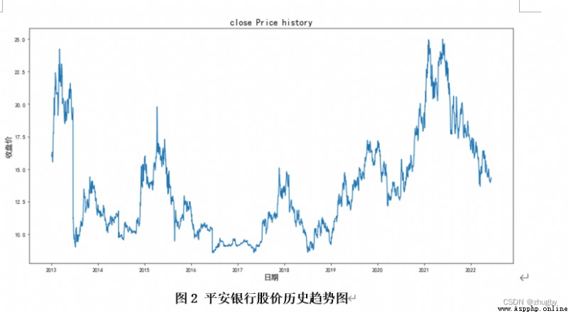
First, observe the trend chart of the closing price :
df['trade_date']= convert_date_from_int(df['trade_date'])
df.index = df['trade_date']
#setting index as date
#plot
plt.rcParams['font.sans-serif'] = ['SimHei']
plt.rcParams['axes.unicode_minus'] = False
plt.figure(figsize=(16,8))
plt.plot(df['close'], label='close price history')
plt.title('close Price history',fontsize=16)
plt.xlabel(' date ',fontsize=14)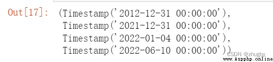
plt.ylabel(' Closing price ',fontsize=14)The prediction of time series data needs to divide the training test set , In this paper 2012-12-31 to 2021-12-31 Ten years of data as a training set , take 2022-01-04 to 2022-06-10 As a test set . As shown in the figure below :
#creating dataframe with date and the target variable
data = df.sort_index(ascending=True, axis=0)
new_data = df[['trade_date', 'close']].sort_index(ascending=True, axis=0)
new_data.head()
#splitting into train and validation
valid = new_data[2187:]
train = new_data[:2187]
Observe the size and start time of the test training set :
new_data.shape, train.shape, valid.shapeoutput:
train['trade_date'].min(), train['trade_date'].max(), valid['trade_date'].min(), valid['trade_date'].max()output:
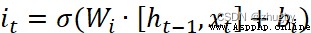
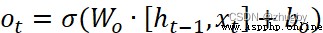
LSTM Model on 1997 Year by year Hochreiter & Schmidhuber [1] Put forward , yes RNN A variant of , Full name Long short-Term Memory, That is, the artificial neural network model of long-term and short-term memory [2]. seeing the name of a thing one thinks of its function , It is a neural network with long-term and short-term information storage capacity . After years of development , Coupled with the continuous improvement of scholars after the upsurge of in-depth learning , At present LSTM The network has formed a relatively systematic and perfect framework , And it is widely used in many fields .
Cyclic neural network (RNN)、BP Neural networks will face the problem of gradient disappearance or gradient explosion caused by back propagation when the network layer is deepened , It is difficult to express long-term dependency . In order to solve this long-term dependence problem ,LSTM In tradition RNN Based on the introduction of the door control unit (gate) To control the transmission of information , Contains three doors : Oblivion gate  , Input gate
  , Output gate
  . Forgetfulness gate determines the last cell state
  How much information needs to be discarded , The input gate decides to save the cell state
  What information about freshmen , The output gate decides at this moment
  Information that needs to be output to the outside [3].
LSTM Processing timing data through three gates , First, through the forgetting door , The mathematical expression of forgetting gate is as follows :

(1)
among , and  Respectively represent the weight and offset parameters of the forgetting gate .
adopt  and
and  Output one 0 To 1 The vector between , Determine how much information about the last cell state needs to be forgotten ,0 Means to discard all ,1 It means to accept all .
Then the information is passed to the input gate , The input gate consists of two parts ,1)sigmoid Activation gets updated status it 2)tanh Activate to get candidate status , The formula is as follows :
(2)

(3)
among , 、
、 Represents the weight parameter ,
 、 Indicates the offset parameter
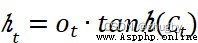
After getting started , Last cell information Updated to , Finally, decide what information to output through the output gate . The output gate also contains two parts ,1)sigmoid layer 2)tanh layer , Unlike the output gate ,sigmoid Layers determine which parts of the cell state to export ,tanh It is worth to adjust the cell state by layer transformation 0-1 Multiply the vector between by the cell state Ct Get the final output . The mathematical expression is as follows :
(4)
(5)
among , representative sigmoid Activate the weight parameter of the function layer , representative sigmoid Activate the offset parameter of the function layer .
 representative sigmoid Activate the output of the function layer ,
 Represents the output of the time memory unit , Implicit state .
The schematic diagram of door control unit is as follows :
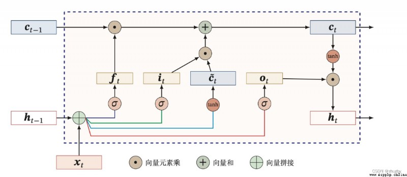
chart 3 LSTM Schematic diagram of door control unit
Put each cell / When the door control unit is connected, it becomes LSTM The overall structure of , As shown in the figure below :
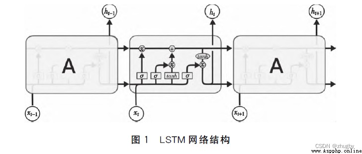
chart 4 LSTM Network structure
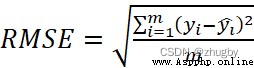
Mean square error is used in this paper RMSE As the index of model evaluation , Mean square error RMSE It measures the difference between the predicted value and the real value of the model , It is often used as a standard to measure the prediction results of machine learning . As formula (1) Shown :
(6)
Calculate the mean square error , have to RMSE=0.5793, Display the prediction results with visual graphics .
combination RMSE Values and graphs ,LSTM The algorithm has a high degree of fitting , Excellent performance in prediction accuracy .
#importing required libraries
from sklearn.preprocessing import MinMaxScaler
from keras.models import Sequential
from keras.layers import Dense, Dropout, LSTM
#setting index
data = df.sort_index(ascending=True, axis=0)
new_data = data[['trade_date', 'close']]
new_data.index = new_data['trade_date']
new_data.drop('trade_date', axis=1, inplace=True)
new_data.head()
#creating train and test sets
dataset = new_data.values
train= dataset[0:2187,:]
valid = dataset[2187:,:]
#converting dataset into x_train and y_train
scaler = MinMaxScaler(feature_range=(0, 1))
scaled_data = scaler.fit_transform(dataset)
x_train, y_train = [], []
for i in range(60,len(train)):
x_train.append(scaled_data[i-60:i,0])
y_train.append(scaled_data[i,0])
x_train, y_train = np.array(x_train), np.array(y_train)
x_train = np.reshape(x_train, (x_train.shape[0],x_train.shape[1],1))
# create and fit the LSTM network
model = Sequential()
model.add(LSTM(units=50, return_sequences=True, input_shape=(x_train.shape[1],1)))
model.add(LSTM(units=50))
model.add(Dense(1))
model.compile(loss='mean_squared_error', optimizer='adam')
model.fit(x_train, y_train, epochs=1, batch_size=1, verbose=1)
#predicting 246 values, using past 60 from the train data
inputs = new_data[len(new_data) - len(valid) - 60:].values
inputs = inputs.reshape(-1,1)
inputs = scaler.transform(inputs)
X_test = []
for i in range(60,inputs.shape[0]):
X_test.append(inputs[i-60:i,0])
X_test = np.array(X_test)
X_test = np.reshape(X_test, (X_test.shape[0],X_test.shape[1],1))
closing_price = model.predict(X_test)
closing_price1 = scaler.inverse_transform(closing_price)
rms=np.sqrt(np.mean(np.power((valid-closing_price1),2)))
rms
#v=new_data[2187:]
valid1['Pre_Lstm'] = closing_price1
train=new_data[:2187]
plt.figure(figsize=(16,8))
plt.plot(train['close'])
plt.plot(valid1['close'],label=' True value ')
plt.plot(valid1['Pre_Lstm'],label=' Predictive value ')
plt.title('LSTM forecast ',fontsize=16)
plt.xlabel(' date ',fontsize=14)
plt.ylabel(' Closing price ',fontsize=14)
plt.legend(loc=0)
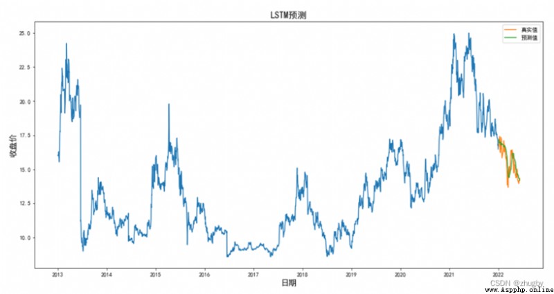
In order to show more clearly lstm Model performance , This paper selects four representative models , Moving average in linear model 、 Linear regression , Traditional machine learning model KNN, Deep learning model LSTM, Four models are used to fit and predict the stock price of Shenzhen Ping An Bank . surface 4 Some predicted values of the four models are shown , chart 12 The comparison shows the stock price prediction trend of the four models , surface 5 Shows four models RSME value .
surface 4 Some test set model predictions
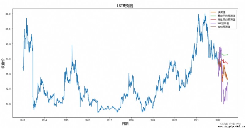 chart 12 Test set 4 Two models predict the trend of stock price comparison
surface 5 Model RSME value
Model
Moving average
Linear regression
KNN
LSTM
RMSE
2.8579
1.7651
2.9326
0.4424
( Because of the space , The implementation code of the other three models is not released , If you need it, you can poke it privately .)
According to the analysis of the results of the comprehensive chart , In terms of accuracy ,LSTM Best performance , The second is linear regression , Moving average method and KNN The algorithm model performs worst ; In predicting the rise and fall trend of the stock price in the future , The performance of moving average and linear regression is slightly better than KNN, The main reason is that they eliminate the volatility of data and show the long-term trend of data . The moving average only relies on the market data of the previous few days to predict the stock price of the next trading day , Linear regression and KNN Rely on date characteristics to fit the regression model , Traditional linear models and machine models do not have the ability to mine the hidden information of data , In the stock market, such fluctuations are large 、 It is difficult to perform satisfactorily on nonlinear data with strong noise .
Some characteristics of the deep learning model make it naturally suitable for processing and predicting financial time series data , Such as :1) The deep learning model is not limited by dimensions , All characteristic data related to dependent variables can be incorporated into the model , Get more perfect characterization ;2) Have good nonlinear fitting ability , It is suitable for fitting time series data with irregular fluctuations ;3) It is not easy to fall into model over fitting and local optimization ;4) Compared with linear regression and traditional machine learning, it does not need manual construction features , Extract hidden features of data through multilayer neural network , Deep network expression ability is stronger . And this article selects LSTM The network has the function of long-term memory , The prediction effect of high noise financial stock data will be better .
because LSTM The model fitting effect is very good , Current use LSTM The model predicts the stock price trend in the short term . Considering the rest of Shenzhen Stock Exchange on weekends , Therefore, it is necessary to exclude weekends and holidays , Used in this article LSTM Model for the future 30 Predict the stock price trend of Ping An Bank within working days , The results are shown in the following figure :
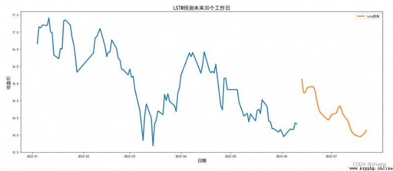
Part of the reason why there are interruptions in the graph is that our real data is cut-off 2020-06-10,6 month 10 It's Friday , The next working day is 6 month 12, Therefore, two days will be left in the middle of the forecast date , On the graph, there is a small interruption .
Observe the stock price trend in the next month or so , Generally speaking, the share price of Ping An Bank will decline in the future . Investors are in 6 month 10 You can choose to increase the stock of Ping An Bank on Friday , Next week, the share price rose to 15.5 Sell at the bottom around , Watch the stock market , Due to the overall downward trend , When the stock market stabilizes, you can consider adding positions slowly .
It is worth noting that , The stock price may be influenced by public opinion 、 The news media also have some force majeure effects , For example, large-scale natural disasters 、 The company's fees are monetized and split 、 The reputation of the company is damaged and so on , These intangible factors that cannot be predicted in advance will have an impact on the stock price . therefore , Investors cannot completely rely on the prediction results given by the model , Pay more attention to the direction of the stock market , Invest cautiously .
1) Realize the extraction and elimination of weekends 30 Day working day date :
import datetime
def date_by_adding_business_days(from_date, add_days):
business_days_to_add = add_days
current_date = from_date
re=[]
while business_days_to_add > 0:
current_date += datetime.timedelta(days=1)
current_date1=current_date.strftime("%Y-%m-%d")
weekday = current_date.weekday()
if weekday < 5: # sunday = 6
re.append(current_date1)
business_days_to_add -= 1
return re
data_pre=date_by_adding_business_days(datetime.date(2022, 6, 10), 30)
2) Model to predict :
dataset = new_data.values
train= dataset
#valid = dataset[2187:,:]
#converting dataset into x_train and y_train
scaler = MinMaxScaler(feature_range=(0, 1))
scaled_data = scaler.fit_transform(dataset)
x_train, y_train = [], []
for i in range(60,len(train)):
x_train.append(scaled_data[i-60:i,0])
y_train.append(scaled_data[i,0])
x_train, y_train = np.array(x_train), np.array(y_train)
x_train = np.reshape(x_train, (x_train.shape[0],x_train.shape[1],1))
model = Sequential()
model.add(LSTM(units=50, return_sequences=True, input_shape=(x_train.shape[1],1)))
model.add(LSTM(units=50))
model.add(Dense(1))
model.compile(loss='mean_squared_error', optimizer='adam')
model.fit(x_train, y_train, epochs=1, batch_size=1, verbose=1)
#predicting 246 values, using past 60 from the train data
inputs = new_data[len(new_data) - 30 - 60:].values
inputs = inputs.reshape(-1,1)
inputs = scaler.transform(inputs)
X_test = []
for i in range(60,inputs.shape[0]):
X_test.append(inputs[i-60:i,0])
X_test = np.array(X_test)
X_test = np.reshape(X_test, (X_test.shape[0],X_test.shape[1],1))
closing_price = model.predict(X_test)
closing_price1 = scaler.inverse_transform(closing_price)
#rms=np.sqrt(np.mean(np.power((valid-closing_price1),2)))
#rms
lstm_pre['date']=data_pre
lstm_pre=pd.DataFrame()
lstm_pre['trade_date']=data_pre
lstm_pre['trade_date']=pd.to_datetime(lstm_pre['trade_date'], format="%Y-%m-%d")
lstm_pre['pred']=closing_price1
lstm_pre.index = lstm_pre['trade_date']
#lstm_pre.drop('trade_date', axis=1, inplace=True)
lstm_pre
#plot
train=new_data[2187:]
plt.figure(figsize=(20,8))
plt.plot(train['close'],linewidth=3)
plt.plot(lstm_pre['pred'],label='lstm forecast ',linewidth=3)
plt.title('LSTM Predicting the future 30 A working day ',fontsize=16)
plt.xlabel(' date ',fontsize=14)
plt.ylabel(' Closing price ',fontsize=14)
plt.legend(loc=0)[1] Hochreiter, S, and J. Schmidhuber. “Long short-term memory.” Neural Computation 9.8(1997):1735-1780.
[2] Liang Yujia , Song Dongfeng . be based on LSTM And emotional analysis of stock forecasts [J]. Technology and innovation ,2021,(21):126-127.
[3] Xu Xuechen , Tian Kan . A new method of stock index prediction based on Emotional Analysis of financial text [J]. The study of quantitative economy, technology and economy ,2021,38(12):124-145.DOI:10.13653/j.cnki.jqte.2021.12.009.