List of articles

• One 、 summary
• Two 、 Algorithm principle
• 3、 ... and 、python Realization
• • 3.1 Build the objective function
  • 3.2 Build the objective function
• Four 、Tips

One 、 summary

Simulated annealing algorithm is a general optimization algorithm , In theory, the algorithm has probabilistic global optimization performance , At present, it has been widely used in engineering , Such as machine learning 、 neural network 、 Signal processing and other fields .

Two 、 Algorithm principle

The idea of simulated annealing algorithm borrows from the annealing principle of solids , When the temperature of the solid is very high , Internal energy is relatively large , The internal particles of a solid are in rapid disordered motion , When the temperature decreases slowly , The internal energy of a solid decreases , The of particles slowly tends to order , Final , When the solid is at room temperature , The internal energy can reach the minimum , here , Particles are the most stable . Simulated annealing algorithm is designed based on this principle .
Simulated annealing algorithm starts from a certain high temperature , Calculate the initial solution at high temperature , Then a disturbance is generated by the preset neighborhood function , So as to get a new state , That is to simulate the disordered motion of particles , Compare the energy in the new and old States , That is, the solution of the objective function . If the energy of the new state is less than that of the old state , Then the state changes ; If the energy of the new state is greater than that of the old state , Then the transformation takes place with a certain probability criterion . When the state is stable , It can be regarded as reaching the optimal solution of the current state , You can start cooling , Continue iteration at the next temperature , Finally, it reaches a stable state of low temperature , The result of simulated annealing algorithm is obtained .
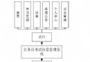
According to the above description , It can be concluded that the calculation steps of simulated annealing algorithm are as follows ：

1. initialization : initial temperature T T T ( Big enough ), Lower temperature limit T min ⁡ T_{\min } Tmin​ ( Sufficiently small ), The initial solution state x x x ( It's the starting point of algorithm iteration ), Every T T T Iterations of values frequency L L L;
2. Yes l = 1 , 2 , … , L l=1,2, \ldots, L l=1,2,…,L Do the first 3 To 6 Step ;
3. New solutions x new.  x new  = x + Δ x ; Δ x x_{\text {new. }} x_{\text {new }}=x+\Delta x ; \Delta x xnew. ​xnew ​=x+Δx;Δx by [ d min ⁡ , d max ⁡ ] \left[d_{\min }, d_{\max }\right] [dmin​,dmax​] Random number between ;
4. Benefit calculation increment Δ f = f ( x n e w ) − f ( x ) \Delta f=f\left(x_{n e w}\right)-f(x) Δf=f(xnew​)−f(x) , among f ( x ) f(x) f(x) For the purpose of optimization ;
5. if Δ f < 0 \Delta f<0 Δf<0 ( If you look for the maximum , Δ f > 0 \Delta f>0 Δf>0 ) received x n e w x_{n e w} xnew​ As a new current solution , Otherwise, with probability exp ⁡ ( − Δ f / ( k T ) ) \exp (-\Delta f /(k T)) exp(−Δf/(kT)) Accept x n e w x_{n e w} xnew​ As new The current solution ;
6. If the termination condition is satisfied, the current solution is output as the optimal solution , End procedure .( The termination condition is usually taken as the termination when several new solutions in succession are not accepted Law ;
7. T T T Gradually reduce , And T > T min ⁡ T>T_{\min } T>Tmin​ , And then turn to 2 Step .

3、 ... and 、python Realization

3.1 Build the objective function

import numpy as np
import matplotlib.pyplot as plt
# Build the objective function 
def aimFunc(x):
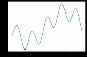
y = 11 * np.sin(x) + 7*np.cos(5*x)
return y
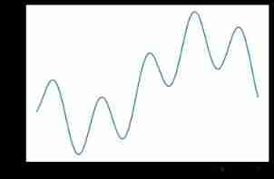
# Show the curve of the objective function in the interval to be solved 
x = np.arange(-3, 3, 0.01)
y = aimFunc(x)
plt.plot(x, y)
plt.show()

3.2 Build the objective function

# Build new location 
def new_x(x, T, x_l, x_h):
# Calculate the new location 
_x_new = x + np.random.uniform(-1, 1) * T
# If the new position exceeds the upper 、 Lower limit , Readjust the position 
if(_x_new < x_l):
_x_new = x - np.random.uniform(0, 1)*(x-x_l)
if(_x_new > x_h):
_x_new = x + np.random.uniform(0, 1)*(x_h-x)
return _x_new
# Definition x The scope of the 
x_l = -3
x_h = 3
# Define the initial temperature 
T = 1000
# Define the number of internal cycles 
N = 20
# Define the initial position 
_x = np.random.uniform(low=x_l, high=x_h)
_y = aimFunc(_x)
# Define the recorder 
_x_track = []
_y_track = []
while T >= 0.001:
for i in range(N):
# Get a new location 
_x_new = new_x(_x, T, x_l, x_h)
# Calculate the function value corresponding to the new position 
_y_new = aimFunc(_x_new)
# Decide whether to accept the new position 
flag_1 = _y_new < _y
flag_2 = np.exp(-(_y_new-_y)/T) > np.random.uniform()
if(flag_1 | flag_2):
_x = _x_new
_y = _y_new
_x_track.append(_x)
_y_track.append(_y)
# Update temperature 
T = T * 0.8
# Show the calculation results 
print(_x)
print(_y)
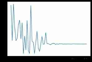
plt.plot(_x_track)
plt.show()
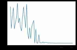
plt.plot(_y_track)
plt.show()
plt.plot(x, y)
plt.scatter(_x, _y, c='r')
plt.show()

Four 、Tips

Simulated annealing algorithm has the following three parameter adjustment problems ：

1. temperature T Initial value setting problem
   temperature T The initial value setting of is one of the important factors affecting the global search performance of simulated annealing algorithm 、 The initial temperature is high , Then it is more likely to search the global optimal solution , But it takes a lot of computing time ; conversely , The calculation time can be saved , However, global search performance may be affected .
2. Annealing speed problem , each T The number of iterations of the value L
   The global search performance of simulated annealing algorithm is also closely related to the annealing speed . Generally speaking , At the same temperature “ to the full ” Search is quite necessary , But it also takes time to calculate . An increase in the number of cycles will inevitably lead to an increase in computational overhead .
3. Temperature management issues
   Temperature management is also one of the problems that simulated annealing algorithm is difficult to deal with . Practical application , Because the practical feasibility of computational complexity must be considered .