Finish today :【OpenCV routine 100 piece 】100. Adaptive local noise reduction filter
Celebrate Jiageng : Python Big white starts from scratch OpenCV Learning lessons -8. Frequency domain image filtering ( On )Welcome to your attention 『OpenCV routine 200 piece 100 piece 』 series , Ongoing update
Welcome to your attention 『Python Small white OpenCV Learning lessons 』 series , Ongoing update
This series is for Python The small white , Start from scratch OpenCV Project practice .
Image filtering is to suppress the noise of the target image while preserving the detailed features of the image as much as possible , It is a common image preprocessing operation .
In frequency domain image processing, the image is first Fourier transformed , Then it is processed in the transform domain , Finally, the inverse Fourier transform is carried out and converted back to the spatial domain .
Frequency domain filtering is the multiplication of the filter transfer function and the corresponding pixel of the Fourier transform of the input image . The concept of filtering in frequency domain is more intuitive , Filter design is also easier . Using fast Fourier transform algorithm , Much faster than spatial convolution .
This paper provides the complete routines and running results of the above algorithms , An application case is used to demonstrate the comprehensive use of a variety of image enhancement methods .
Filtering usually refers to filtering or suppressing the components of a specific frequency in the image . Image filtering is to suppress the noise of the target image while preserving the detailed features of the image as much as possible , It is a common image preprocessing operation .
Image filtering can be carried out not only in spatial domain, but also in frequency domain . Spatial filtering is the combination of image and various spatial filters ( Templates 、 nucleus ) Convolution of , The Fourier transform of spatial convolution is the product of the corresponding transform in the frequency domain , Therefore, frequency domain filtering is a frequency domain filter ( Transfer function ) Multiplied by the Fourier transform of the image .
Frequency domain image filtering , First, Fourier transform the image , Then it is processed in the transform domain , Finally, the inverse Fourier transform is carried out and converted back to the spatial domain .
The spatial domain filter and the frequency domain filter form a Fourier transform pair :
f ( x , y ) ⊗ h ( x , y ) ⇔ F ( u , v ) H ( u , v ) f ( x , y ) h ( x , y ) ⇔ F ( u , v ) ⊗ H ( u , v ) f(x,y) \otimes h(x,y) \Leftrightarrow F(u,v)H(u,v) \\f(x,y) h(x,y) \Leftrightarrow F(u,v) \otimes H(u,v) f(x,y)⊗h(x,y)⇔F(u,v)H(u,v)f(x,y)h(x,y)⇔F(u,v)⊗H(u,v)
in other words , Spatial domain filter and frequency domain filter are actually corresponding to each other , It is more convenient for some spatial domain filters to be realized by Fourier transform in frequency domain 、 Faster . for example , Laplace filter in space domain is high pass filter in frequency domain .
Fourier series (Fourier series) In number theory 、 Combinatorial mathematics 、 signal processing 、 probability theory 、 statistical 、 cryptography 、 acoustics 、 Optics and other fields have a wide range of applications .
The Fourier series formula indicates that , Any periodic function can be expressed as a sine function of different frequencies and / Or the weighted sum of cosine functions :
f ( t ) = A 0 + ∑ n = 1 ∞ A n s i n ( n ω t + ψ n ) = A 0 + ∑ n = 1 ∞ [ a n c o s ( n ω t ) + b n s i n ( n ω t ) ] \begin{aligned} f(t) &= A_0 + \sum^{\infty}_{n=1} A_n sin(n \omega t + \psi _n)\\ &= A_0 + \sum^{\infty}_{n=1} [a_n cos(n \omega t) + b_n sin(n \omega t)] \end{aligned} f(t)=A0+n=1∑∞Ansin(nωt+ψn)=A0+n=1∑∞[ancos(nωt)+bnsin(nωt)]
This sum is Fourier series .
Further , Any aperiodic function can also be expressed as sinusoidal functions of different frequencies and / Or the integral of the cosine function multiplied by the weighting function :
F ( ω ) = ∫ − ∞ + ∞ f ( t ) e − j ω t d t f ( t ) = 1 2 π ∫ − ∞ + ∞ F ( ω ) e j ω t d ω \begin{aligned} F(\omega) &= \int_{-\infty}^{+\infty} f(t) e^{-j\omega t} dt\\ f(t) &= \frac{1}{2 \pi} \int_{-\infty}^{+\infty} F(\omega) e^{j\omega t} d \omega \end{aligned} F(ω)f(t)=∫−∞+∞f(t)e−jωtdt=2π1∫−∞+∞F(ω)ejωtdω
This formula is Fourier transform (Fourier transform ) And inverse transformation .
* The sufficient condition for the existence of Fourier transform is :f(t) The integral of the absolute value of is finite , In signal processing 、 In the field of image processing, this condition can be met .
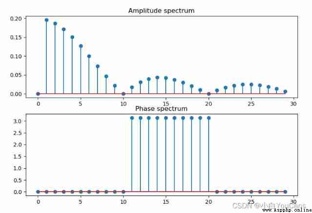
 # 8.1: Continuous Fourier series of periodic signals
from scipy import integrate
nf = 30
T = 10
tao = 1.0
y = 1
k = np.arange(0, nf)
an = np.zeros(nf)
bn = np.zeros(nf)
amp = np.zeros(nf)
pha = np.zeros(nf)
half0, err0 = integrate.quad(lambda t: y, -tao/2, tao/2)
an[0] = 2 * half0 / T
for n in range(1, nf):
half1, err1 = integrate.quad(lambda t: 2*y * np.cos(2.0/T * np.pi * n * t), -tao/2, tao/2)
an[n] = half1 / 10
half2, err2 = integrate.quad(lambda t: 2*y * np.sin(2.0/T * np.pi * n * t), -tao/2, tao/2)
bn[n] = half2 / 10
amp[n] = np.sqrt(an[n]**2 + bn[n]**2)
for i in range(0, nf):
pha[i] = 0.0 if an[i]>=0 else np.pi
plt.figure(figsize=(9, 6))
plt.subplot(211), plt.title("Amplitude spectrum"), plt.stem(k, amp)
plt.subplot(212), plt.title("Phase spectrum"), plt.stem(k, pha)
plt.show()
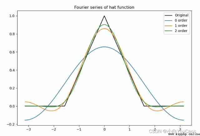
 # 8.2: Discontinuous Fourier coefficients
dx = 0.001
x = np.pi * np.arange(-1+dx, 1+dx, dx)
n = len(x)
nquart = int(np.floor(n/4))
f = np.zeros_like(x)
f[nquart: 2*nquart] = (4/n) * np.arange(1, nquart+1)
f[2*nquart: 3*nquart] = np.ones(nquart) - (4/n) * np.arange(0, nquart)
plt.figure(figsize=(9, 6))
plt.title("Fourier series of hat function")
plt.plot(x, f, '-', color='k',label="Original")
# Compute Fourier series
A0 = np.sum(f * np.ones_like(x)) * dx
fFS = A0 / 2
orders = 3
A = np.zeros(orders)
B = np.zeros(orders)
for k in range(orders):
A[k] = np.sum(f * np.cos(np.pi * (k+1) * x / np.pi)) * dx # Inner product
B[k] = np.sum(f * np.sin(np.pi * (k+1) * x / np.pi)) * dx
fFS = fFS + A[k] * np.cos((k + 1) * np.pi * x / np.pi) + B[k] * np.sin((k + 1) * np.pi * x / np.pi)
plt.plot(x, fFS, '-', label="{} order".format(k))
print('Line ', k, ': A = ', A[k], ' B = ', B[k], fFS.shape)
plt.legend(loc="upper right")
plt.show()
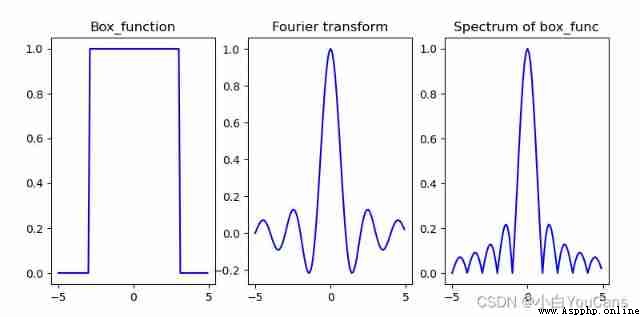
Take one-dimensional box function as an example , Its Fourier transform is :
F ( ω ) = ∫ − ∞ + ∞ f ( t ) e − j ω t d t = ∫ − π π f ( t ) e − j ω t d t = s i n ( ω ) ω \begin{aligned} F(\omega) &= \int_{-\infty}^{+\infty} f(t) e^{-j\omega t} dt\\ &= \int_{-\pi}^{\pi} f(t) e^{-j\omega t} dt\\ &= \frac{sin(\omega)}{\omega} \end{aligned} F(ω)=∫−∞+∞f(t)e−jωtdt=∫−ππf(t)e−jωtdt=ωsin(ω)
 # 8.3: Fourier transform of one-dimensional continuous function ( Box functions )
# Box functions (Box_function)
x = np.arange(-5, 5, 0.1)
w = 2 * np.pi
halfW = w / 2
y = np.where(x, x > -halfW, 0)
y = np.where(x < halfW, y, 0)
plt.figure(figsize=(9, 4))
plt.subplot(131), plt.title("Box_function")
plt.plot(x, y, '-b')
plt.subplot(132), plt.title("Fourier transform")
fu = np.sinc(x)
plt.plot(x, fu, '-b')
plt.subplot(133), plt.title("Spectrum of box_func")
fu = abs(fu)
plt.plot(x, fu, '-b')
plt.show()
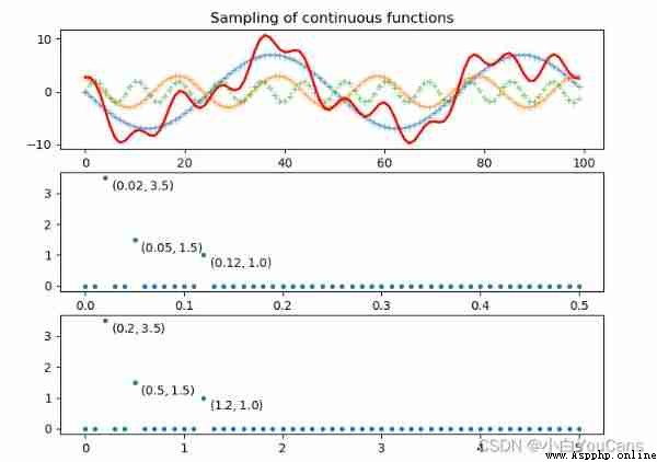
Continuous functions must be sampled and quantized into discrete functions , Can be processed by computer .
Consider a continuous function f ( t ) f(t) f(t), In terms of independent variables t Evenly spaced Δ T \Delta T ΔT Sample functions , Any sampling value in the sampling sequence is :
f k = ∫ − ∞ + ∞ f ( t ) δ ( t − k Δ T ) d t = f ( k Δ T ) f_k = \int_{-\infty}^{+\infty} f(t) \delta (t-k \Delta T) dt = f(k \Delta T) fk=∫−∞+∞f(t)δ(t−kΔT)dt=f(kΔT)
The Fourier transform of the sampled function is :
F ~ ( μ ) = ( F ⋆ S ) ( μ ) = ∫ − ∞ + ∞ F ( τ ) S ( μ − τ ) d τ = 1 Δ T ∑ n = − ∞ ∞ F ( μ − n Δ T ) \begin{aligned} \tilde{F}(\mu) &= (F \star S) (\mu) \\ &= \int_{-\infty}^{+\infty} F(\tau) S(\mu-\tau) d \tau\\ &= \frac{1}{\Delta T} \sum_{n=-\infty}^{\infty}F(\mu-\frac{n}{\Delta T}) \end{aligned} F~(μ)=(F⋆S)(μ)=∫−∞+∞F(τ)S(μ−τ)dτ=ΔT1n=−∞∑∞F(μ−ΔTn)
Shannon (Shannon) The sampling theorem states , For a continuous signal , Use a frequency greater than the maximum frequency of the signal 2 Times the sampling rate , The valid information of the signal will not be lost . Or say , With 1 / Δ T 1/\Delta T 1/ΔT What is the maximum frequency of the sampling rate to the signal sampling point μ m a x = 1 / 2 Δ T \mu_{max}=1/2\Delta T μmax=1/2ΔT .
 # 8.4: Sampling of continuous functions
# Defined function , Used to calculate the frequency of all basis vectors
def gen_freq(N, fs):
k = np.arange(0, np.floor(N/2) + 1, 1)
return (k * fs) / N
T = 100
# Define multiple fundamental frequency signals with different frequencies
fk = [2/T, 5/T, 12/T] # frequency
A = [7, 3, 2] # The amplitude
phi = [np.pi, 2, 2*np.pi] # Initial phase
n = np.arange(T)
s0 = A[0] * np.sin(2 * np.pi * fk[0] * n + phi[0])
s1 = A[1] * np.sin(2 * np.pi * fk[1] * n + phi[1])
s2 = A[2] * np.sin(2 * np.pi * fk[2] * n + phi[2])
s = s0 + s1 + s2 # Superimpose to generate mixed signal
g = np.fft.rfft(s) # The Fourier transform
plt.figure(figsize=(8, 6))
plt.subplot(311)
plt.plot(n, s0, n, s1, n, s2, ':', marker='+', alpha=0.5)
plt.plot(n, s, 'r-', lw=2)
plt.title("Sampling of continuous functions")
plt.subplot(312)
fs = 1 # The sampling interval is 1
freq = gen_freq(T, fs=fs) # Calculate the frequency sequence
ck = np.abs(g) / T # Calculate the amplitude
plt.plot(freq, ck, '.') # frequency - Amplitude diagram
for f in fk:
ck0 = round(ck[np.where(freq==f*fs)][0], 1)
plt.annotate('$({},{})$'.format(f*fs, ck0), xy=(f*fs, ck0), xytext=(5, -10), textcoords='offset points')
plt.subplot(313)
fs = 10 # The sampling interval is 10
freq = gen_freq(T, fs=fs) # Calculate the frequency sequence
ck = np.abs(g) / T # Calculate the amplitude
plt.plot(freq, ck, '.') # frequency - Amplitude diagram
for f in fk:
ck0 = round(ck[np.where(freq==f*fs)][0], 1)
plt.annotate('$({},{})$'.format(f*fs, ck0), xy=(f*fs, ck0), xytext=(5, -10), textcoords='offset points')
plt.show()
Both digital signal and digital image are discrete variables obtained by sampling .
The data after sampling the transformation of the original function
F ~ ( μ ) = ∫ − ∞ + ∞ f ~ ( t ) e − j 2 π μ t d t = ∫ − ∞ + ∞ ∑ n = − ∞ ∞ f ( t ) δ ( t − n Δ T ) e − j 2 π μ t d t = ∑ n = − ∞ ∞ ∫ − ∞ + ∞ f ( t ) δ ( t − n Δ T ) e − j 2 π μ t d t = ∑ n = − ∞ ∞ f n e − j 2 π μ n Δ T \begin{aligned} \tilde{F}(\mu) &= \int_{-\infty}^{+\infty} \tilde{f}(t) e^{-j 2 \pi \mu t} dt\\ &= \int_{-\infty}^{+\infty} \sum_{n=-\infty}^{\infty} f(t) \delta (t-n{\Delta T}) e^{-j 2 \pi \mu t} dt\\ &= \sum_{n=-\infty}^{\infty} \int_{-\infty}^{+\infty} f(t) \delta (t-n{\Delta T}) e^{-j 2 \pi \mu t} dt\\ &= \sum_{n=-\infty}^{\infty} f_n e^{-j 2 \pi \mu n{\Delta T}}\\ \end{aligned} F~(μ)=∫−∞+∞f~(t)e−j2πμtdt=∫−∞+∞n=−∞∑∞f(t)δ(t−nΔT)e−j2πμtdt=n=−∞∑∞∫−∞+∞f(t)δ(t−nΔT)e−j2πμtdt=n=−∞∑∞fne−j2πμnΔT
When the sampling frequency is μ = m / M Δ T \mu = m/M \Delta T μ=m/MΔT when , The discrete Fourier transform can be obtained (DFT) And the inverse transformation formula is :
F m = ∑ n = 0 M − 1 f n e − j 2 π μ m n / M , m = 0 , . . . M − 1 f n = 1 M ∑ m = 0 M − 1 F m e j 2 π μ m n / M , n = 0 , . . . M − 1 \begin{aligned} F_m &= \sum_{n=0}^{M-1} f_n e^{-j\ 2\pi \mu mn/M}, &m=0,...M-1\\ f_n &= \frac{1}{M} \sum_{m=0}^{M-1} F_m e^{j\ 2\pi \mu mn/M}, &n=0,...M-1 \end{aligned} Fmfn=n=0∑M−1fne−j 2πμmn/M,=M1m=0∑M−1Fmej 2πμmn/M,m=0,...M−1n=0,...M−1
Because any periodic or aperiodic function can be expressed as the sum of sine function and cosine function of different frequencies , Therefore, the function characteristics expressed by Fourier transform can be reconstructed by inverse Fourier transform , And you won't lose any information . This is the mathematical basis of frequency domain image processing .
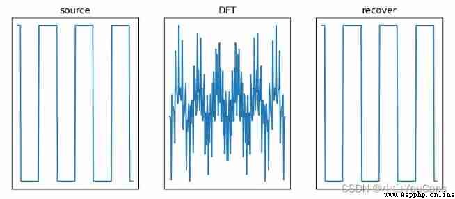
Discrete Fourier transform Is to decompose the discrete signal into a series of discrete trigonometric function components , Each trigonometric function component has a corresponding amplitude A、 frequency f And phase φ \varphi φ. All the original discrete components can be superimposed .
In image processing , Usually use x , y x, y x,y Represents a discrete space coordinate variable , use u , v u,v u,v Represents a discrete variable in the frequency domain . Therefore, the one-dimensional discrete Fourier transform is expressed as :
F ( u ) = ∑ x = 0 M − 1 f ( x ) e − j 2 π u x / M , u = 0 , . . . M − 1 f ( x ) = 1 M ∑ u = 0 M − 1 F ( u ) e j 2 π u x / M , x = 0 , . . . M − 1 \begin{aligned} F(u) &= \sum_{x=0}^{M-1} f(x) e^{-j\ 2\pi u x/M}, &u=0,...M-1\\ f(x) &= \frac{1}{M} \sum_{u=0}^{M-1} F(u) e^{j\ 2\pi u x/M}, &x=0,...M-1 \end{aligned} F(u)f(x)=x=0∑M−1f(x)e−j 2πux/M,=M1u=0∑M−1F(u)ej 2πux/M,u=0,...M−1x=0,...M−1
 # 8.6: One dimensional discrete Fourier transform
# Generate square wave signal
N = 200
t = np.linspace(-10, 10, N)
dt = t[1] - t[0]
sint = np.sin(t)
sig = np.sign(sint)
fig = plt.figure(figsize=(10, 4))
plt.subplot(131), plt.title("source"), plt.xticks([]), plt.yticks([])
plt.plot(t, sig)
# Discrete Fourier transform
fft = np.fft.fft(sig, N) # Discrete Fourier transform
fftshift = np.fft.fftshift(fft) # Symmetrical translation
amp = abs(fftshift) / len(fft) # amplitude
pha = np.angle(fftshift) # phase
fre = np.fft.fftshift(np.fft.fftfreq(d=dt, n=N)) # frequency
plt.subplot(132), plt.title("DFT"), plt.xticks([]), plt.yticks([])
plt.plot(t, fft)
# Signal recovery
recover = np.zeros(N)
for a, p, f in zip(amp, pha, fre):
sigCos = a * np.cos(2 * np.pi * f * np.arange(N) * dt + p) # According to the amplitude , phase , Frequency construction trigonometric function
recover += sigCos # Add up all these trigonometric functions
plt.subplot(133), plt.title("recover"), plt.xticks([]), plt.yticks([])
plt.plot(t, recover)
plt.show()
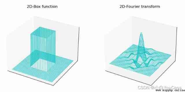
set up f ( t , z ) f(t,z) f(t,z) Is a two-dimensional continuous variable t , z t, z t,z The continuous function of , Then the two-dimensional continuous Fourier transform and inverse transform are :
F ( μ , ν ) = ∫ − ∞ + ∞ ∫ − ∞ + ∞ f ( t , z ) e − j 2 π ( μ t + ν z ) d t d z f ( t , z ) = ∫ − ∞ + ∞ ∫ − ∞ + ∞ F ( μ , ν ) e j 2 π ( μ t + ν z ) d μ d ν \begin{aligned} F(\mu,\nu) &= \int_{-\infty}^{+\infty} \int_{-\infty}^{+\infty} f(t,z) e^{-j 2\pi (\mu t + \nu z)} dt \ dz\\ f(t,z) &= \int_{-\infty}^{+\infty} \int_{-\infty}^{+\infty} F(\mu,\nu) e^{j 2\pi (\mu t + \nu z)} d\mu \ d\nu \end{aligned} F(μ,ν)f(t,z)=∫−∞+∞∫−∞+∞f(t,z)e−j2π(μt+νz)dt dz=∫−∞+∞∫−∞+∞F(μ,ν)ej2π(μt+νz)dμ dν
For image processing , Type in the t , z t, z t,z Represents a continuous spatial variable , μ , ν \mu, \nu μ,ν Represents a continuous frequency variable .
Take box functions as an example , Its Fourier transform is :
F ( μ , ν ) = ∫ − ∞ + ∞ ∫ − ∞ + ∞ f ( t , z ) e − j 2 π ( μ t + ν z ) d t d z = ∫ − T / 2 + T / 2 ∫ − Z / 2 + Z / 2 A e − j 2 π ( μ t + ν z ) d t d z = A T Z [ s i n ( π μ T ) π μ T ] [ s i n ( π ν Z ) π ν Z ] \begin{aligned} F(\mu,\nu) &= \int_{-\infty}^{+\infty} \int_{-\infty}^{+\infty} f(t,z) e^{-j 2\pi (\mu t + \nu z)} dt \ dz\\ &= \int_{-T/2}^{+T/2} \int_{-Z/2}^{+Z/2} A e^{-j 2\pi (\mu t + \nu z)} dt \ dz\\ &= ATZ[\frac{sin(\pi \mu T)}{\pi \mu T}][\frac{sin(\pi \nu Z)}{\pi \nu Z}] \end{aligned} F(μ,ν)=∫−∞+∞∫−∞+∞f(t,z)e−j2π(μt+νz)dt dz=∫−T/2+T/2∫−Z/2+Z/2Ae−j2π(μt+νz)dt dz=ATZ[πμTsin(πμT)][πνZsin(πνZ)]
 # 8.7: Fourier transform of two-dimensional continuous function ( Two dimensional box function )
# Two dimensional box function (2D-Box_function)
t = np.arange(-5, 5, 0.1) # start, end, step
z = np.arange(-5, 5, 0.1)
height, width = len(t), len(z)
tt, zz = np.meshgrid(t, z) # One dimensional arrays xnew, ynew Convert to grid point set ( Two dimensional array )
f = np.zeros([len(t), len(z)]) # initialization , Zeroing
f[30:70, 30:70] = 1 # Two dimensional box function
fu = np.sinc(t)
fv = np.sinc(z)
fuv = np.outer(np.sinc(t), np.sinc(z)) # Calculate the Continuous Fourier transform from the formula
print(fu.shape, fv.shape, fuv.shape)
fig = plt.figure(figsize=(10, 6))
ax1 = plt.subplot(121, projection='3d')
ax1.set_title("2D-Box function")
ax1.plot_wireframe(tt, zz, f, rstride=2, cstride=2, linewidth=0.5, color='c')
ax1.set_xticks([]), ax1.set_yticks([]), ax1.set_zticks([])
ax2 = plt.subplot(122, projection='3d')
ax2.set_title("2D-Fourier transform")
ax2.plot_wireframe(tt, zz, fuv, rstride=2, cstride=2, linewidth=0.5, color='c')
ax2.set_xticks([]), ax2.set_yticks([]), ax2.set_zticks([])
plt.show()
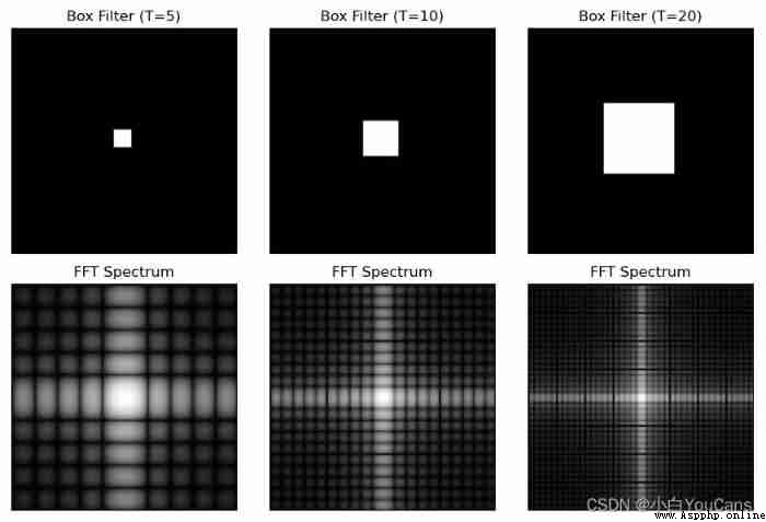
 # 8.8: Fourier transform of two-dimensional continuous function ( Box functions with different parameters )
# Two dimensional box function (2D-Box_function)
height, width = 128, 128
m = int((height - 1) / 2)
n = int((width - 1) / 2)
fig = plt.figure(figsize=(9, 6))
T = [5, 10, 20]
print(len(T))
for i in range(len(T)):
f = np.zeros([height, width]) # initialization , Zeroing
f[m-T[i]:m+T[i], n-T[i]:n+T[i]] = 1 # Box functions of different sizes
fft = np.fft.fft2(f)
shift_fft = np.fft.fftshift(fft)
amp = np.log(1 + np.abs(shift_fft))
plt.subplot(2,len(T),i+1), plt.xticks([]), plt.yticks([])
plt.imshow(f, "gray"), plt.title("Box Filter (T={})".format(T[i]))
#
plt.subplot(2,len(T),len(T)+i+1), plt.xticks([]), plt.yticks([])
plt.imshow(amp, "gray"), plt.title("FFT Spectrum")
plt.tight_layout()
plt.show()
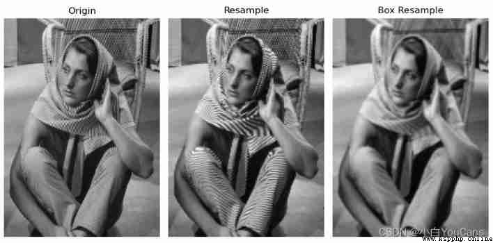
Because a function cannot be sampled indefinitely , Therefore, aliasing always occurs in digital images .
Aliasing is divided into spatial aliasing and temporal aliasing . Spatial aliasing is caused by under sampling , It is more obvious in unfamiliar and repeated images . Time aliasing is related to the time interval of images in dynamic image sequence , As if the spokes were reversed “ Wheel effect ”.
The main problem of spatial aliasing is the introduction of artifacts , That is, the line sawtooth that does not appear in the original image 、 False highlights and frequency patterns .
Aliasing will be introduced when scaling the image . Image magnification can be considered oversampling , Use bilinear 、 Bicubic interpolation can reduce aliasing in image magnification . Image reduction can be regarded as under sampling , Aliasing is usually more severe .
To reduce aliasing , Before resampling, a low-pass filter should be used to smooth , To attenuate the high-frequency component of the image , It can effectively suppress aliasing , But the sharpness of the image has also decreased .
 # 8.9: Anti aliasing of images
imgGray = cv2.imread("../images/Fig0417a.tif", flags=0) # flags=0 Read as grayscale image
height, width = imgGray.shape[:2] # The height and width of the picture
# First reduce the image , Then enlarge the image
imgZoom1 = cv2.resize(imgGray, (int(0.33*width), int(0.33*height)))
imgZoom2 = cv2.resize(imgZoom1, None, fx=3, fy=3, interpolation=cv2.INTER_AREA)
# First, the original image 5x5 Low pass filtering , Zoom out again , Then enlarge the image
kSize = (5, 5)
imgBoxFilter = cv2.boxFilter(imgGray, -1, kSize) # cv2.boxFilter Method
imgZoom3 = cv2.resize(imgBoxFilter, (int(0.33*width), int(0.33*height)))
imgZoom4 = cv2.resize(imgZoom3, None, fx=3, fy=3, interpolation=cv2.INTER_AREA)
fig = plt.figure(figsize=(9,5))
plt.subplot(131), plt.axis('off'), plt.title("Origin")
plt.imshow(imgGray, cmap='gray')
plt.subplot(132), plt.axis('off'), plt.title("Resample")
plt.imshow(imgZoom2, cmap='gray')
plt.subplot(133), plt.axis('off'), plt.title("Box Resample")
plt.imshow(imgZoom4, cmap='gray')
plt.tight_layout()
plt.show()
For two-dimensional image processing , Usually use x , y x, y x,y Represents a discrete space coordinate variable , use u , v u,v u,v Represents a discrete variable in the frequency domain . Two dimensional discrete Fourier transform (DFT) And inverse transformation (IDFT) by :
F ( u , v ) = ∑ x = 0 M − 1 ∑ y = 0 N − 1 f ( x , y ) e − j 2 π ( u x / M + v y / N ) f ( x , y ) = 1 M N ∑ u = 0 M − 1 ∑ v = 0 N − 1 F ( u , v ) e j 2 π ( u x / M + v y / N ) \begin{aligned} F(u,v) &= \sum_{x=0}^{M-1} \sum_{y=0}^{N-1} f(x,y) e^{-j 2\pi (ux/M+vy/N)}\\ f(x,y) &= \frac{1}{MN} \sum_{u=0}^{M-1} \sum_{v=0}^{N-1} F(u,v) e^{j 2\pi (ux/M+vy/N)} \end{aligned} F(u,v)f(x,y)=x=0∑M−1y=0∑N−1f(x,y)e−j2π(ux/M+vy/N)=MN1u=0∑M−1v=0∑N−1F(u,v)ej2π(ux/M+vy/N)
Two dimensional discrete Fourier transform can also be expressed in polar coordinates :
F ( u , v ) = R ( u , v ) + j I ( u , v ) = ∣ F ( u , v ) ∣ e j ϕ ( u , v ) F(u,v) = R(u,v) + j I(u,v) = |F(u,v)| e^{j \phi (u,v)} F(u,v)=R(u,v)+jI(u,v)=∣F(u,v)∣ejϕ(u,v)
Fourier spectrum (Fourier spectrum) by :
∣ F ( u , v ) ∣ = [ R 2 ( u , v ) + I 2 ( u , v ) ] 1 / 2 |F(u,v)| = [R^2(u,v) + I^2(u,v)]^{1/2} ∣F(u,v)∣=[R2(u,v)+I2(u,v)]1/2
Fourier phase spectrum (Fourier phase spectrum) by :
ϕ ( u , v ) = a r c t a n [ I ( u , v ) / R ( u , v ) ] \phi (u,v) = arctan[I(u,v)/R(u,v)] ϕ(u,v)=arctan[I(u,v)/R(u,v)]
Fourier power spectrum (Fourier power spectrum) by :
P ( u , v ) = ∣ F ( u , v ) ∣ 2 = R 2 ( u , v ) + I 2 ( u , v ) P(u,v) = |F(u,v)|^2 = R^2(u,v) + I^2(u,v) P(u,v)=∣F(u,v)∣2=R2(u,v)+I2(u,v)
Spatial sampling and frequency interval correspond to each other , The interval between discrete variables corresponding to the frequency domain is : Δ u = 1 / M Δ T , Δ v = 1 / N Δ Z \Delta u = 1/M \Delta T,\Delta v = 1/N \Delta Z Δu=1/MΔT,Δv=1/NΔZ. namely : The interval between samples in the frequency domain , It is inversely proportional to the product of the interval between spatial samples and the number of samples .
Space domain filter and frequency domain filter also correspond to each other , The two-dimensional convolution theorem is the link to establish the equivalent relationship between spatial domain and frequency domain filtering :
( f ⋆ h ) ( x , y ) ⇔ ( F ⋅ H ) ( u , v ) (f \star h)(x,y) \Leftrightarrow (F \cdot H)(u,v) (f⋆h)(x,y)⇔(F⋅H)(u,v)
This shows that F and H Namely f and h The Fourier transform of ;f and h Fourier transform of spatial convolution , Is the product of their transformations .
therefore , Calculate the spatial convolution of two functions , It can be calculated directly in the spatial domain , It can also be calculated in the frequency domain : First calculate the Fourier transform of each function , Multiply the two transformations , Finally, the inverse Fourier transform is carried out and converted back to the spatial domain .
in other words , Spatial domain filter and frequency domain filter are actually corresponding to each other , It is more convenient for some spatial domain filters to be realized by Fourier transform in frequency domain 、 Faster .
Numpy Medium np.fft.fft2() Function can realize the Fourier transform of the image .
Function description :
numpy.fft.fft2(a, s=None, axes=(- 2, - 1), norm=None) → out
Parameter description :
matters needing attention :
after np.fft.fft2() Function to realize the picture spectrum information obtained by Fourier transform , The maximum value of the amplitude spectrum ( Low frequency component ) In the upper left corner (0,0) It's about . For the convenience of observation , Usually use np.fft.fftshift() The function moves the low-frequency component to the center of the frequency-domain image .
Function description :
numpy.fft.fftshift(x, axes=None) → y
Parameter description :
 # 8.10:Numpy Realize two-dimensional discrete Fourier transform
normalize = lambda x: (x - x.min()) / (x.max() - x.min() + 1e-6)
imgGray = cv2.imread("../images/Fig0424a.tif", flags=0) # flags=0 Read as grayscale image
# imgGray = cv2.imread("../images/imgBall.png", flags=1) # flags=0 Read as grayscale image
# The Fourier transform
# fft = np.fft.fft2(imgGray.astype(np.float32))
fft = np.fft.fft2(imgGray) # np.fft.fft2 Fourier transform
# Decentralization , Calculate the amplitude spectrum and phase spectrum
ampSpectrum = np.sqrt(np.power(fft.real, 2) + np.power(fft.imag, 2)) # Amplitude spectrum
print("ampSpectrum max={}, min={}".format(ampSpectrum.max(), ampSpectrum.min()))
# phase = np.arctan2(fft.imag, fft.real) # Calculate the phase angle ( Radian system )
# phiSpectrum = phase / np.pi*180 # Convert the phase angle to [-180, 180]
phiSpectrum = np.angle(fft)
# Centralization , Move the low-frequency component to the center of the frequency domain image
fftShift = np.fft.fftshift(fft) # Move the low-frequency component to the center of the frequency domain image
# The amplitude spectrum after centralization
ampSpeShift = np.sqrt(np.power(fftShift.real, 2) + np.power(fftShift.imag, 2))
ampShiftNorm = np.uint8(normalize(ampSpeShift)*255) # Owned by one becomes [0,255]
# Logarithmic transformation of amplitude spectrum
ampSpeLog = np.log(1 + ampSpeShift) # The amplitude spectrum is logarithmically transformed for easy display
ampSpeLog = np.uint8(normalize(ampSpeLog)*255) # Owned by one becomes [0,255]
# np.fft.ifft2 Realize the inverse Fourier transform of the image
invShift = np.fft.ifftshift(fftShift) # Switch the low-frequency reversal back to the four corners of the image
imgIfft = np.fft.ifft2(invShift) # Inverse Fourier transform , The return value is a complex array
imgRebuild = np.abs(imgIfft) # Adjust the complex array to gray space
plt.figure(figsize=(9, 6))
plt.subplot(231), plt.title("Original image"), plt.axis('off')
plt.imshow(imgGray, cmap='gray')
plt.subplot(232), plt.title("FFT phase spectrum"), plt.axis('off')
plt.imshow(phiSpectrum, cmap='gray')
plt.subplot(233), plt.title("Rebuild image with IFFT"), plt.axis('off')
plt.imshow(imgRebuild, cmap='gray')
plt.subplot(234), plt.title("FFT amplitude spectrum"), plt.axis('off')
plt.imshow(ampSpectrum, cmap='gray')
plt.subplot(235), plt.title("FFT-shift amplitude"), plt.axis('off')
plt.imshow(ampSpeShift, cmap='gray')
plt.subplot(236), plt.title("Log-trans of FFT amp"), plt.axis('off')
plt.imshow(ampSpeLog, cmap='gray')
plt.tight_layout()
plt.show()
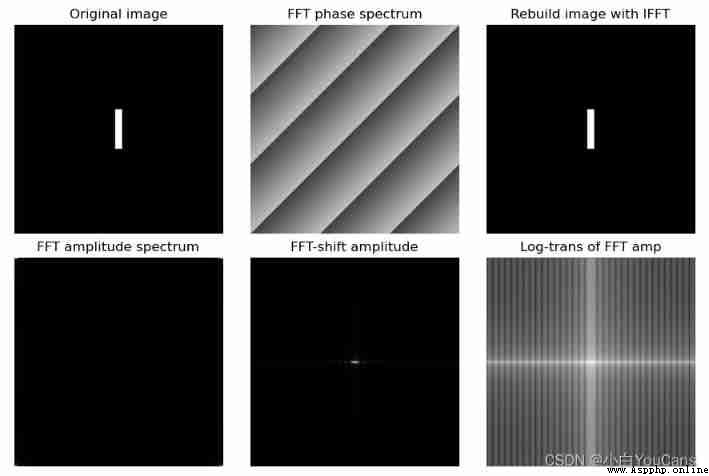
Program description :
The uncentralized amplitude spectrum in the figure (FFT amp spe) It's not completely black , There are tiny bright areas at the four corners of the image , But it's hard to see , This is also the centralization of the amplitude spectrum (fftShift) Why .
Use OpenCV Medium cv.dft() Function can also realize the Fourier transform of the image ,cv.idft() Function to realize the inverse Fourier transform of image .
Function description :
 cv.dft(src[, dst[, flags[, nonzeroRows]]]) → dst
cv.idft(src[, dst[, flags[, nonzeroRows]]]) → dst
Parameter description :
matters needing attention :
Convert the identifier to cv.DFT_COMPLEX_OUTPUT when ,cv.dft() The output of the function is 2 A two-dimensional array of channels , Use cv.magnitude() Function can calculate the amplitude of two-dimensional vector .
Function description :
cv.magnitude(x, y[, magnitude]) → dst
Parameter description :
d s t ( I ) = x ( I ) 2 + y ( I ) 2 dst(I) = \sqrt{x(I)^2 + y(I)^2} dst(I)=x(I)2+y(I)2
The value range of Fourier transform and related operations may not be suitable for image display , It needs to be normalized . OpenCV Medium cv.normalize() Function can realize image normalization .
Function description :
cv.normalize(src, dst[, alpha[, beta[, norm_type[, dtype[, mask]]]]]) → dst
Parameter description :
In theory, Fourier transform needs O ( M N ) 2 O(MN)^2 O(MN)2 Times operation , It's very time consuming ; The fast Fourier transform only needs O ( M N l o g ( M N ) ) O(MN log (MN)) O(MNlog(MN)) One operation can complete .
OpenCV Fourier transform function in cv.dft() The number of rows and columns can be decomposed into 2 p ∗ 3 q ∗ 5 r 2^p * 3^q * 5^r 2p∗3q∗5r The computational performance of the matrix is the best . In order to improve the performance of computation , You can complement the right and bottom of the original matrix 0, To satisfy this decomposition condition .OpenCV Medium cv.getOptimalDFTSize() Function can achieve the optimal image DFT Size expansion , Apply to cv.dft() and np.fft.fft2().
Function description :
cv.getOptimalDFTSize(versize) → retval
Parameter description :
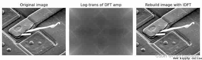
 # 8.11:OpenCV Realize the discrete Fourier transform of two-dimensional image
imgGray = cv2.imread("../images/Fig0424a.tif", flags=0) # flags=0 Read as grayscale image
# cv2.dft Realize Fourier transform of image
imgFloat32 = np.float32(imgGray) # Convert the image to float32
dft = cv2.dft(imgFloat32, flags=cv2.DFT_COMPLEX_OUTPUT) # The Fourier transform
dftShift = np.fft.fftshift(dft) # Move the low-frequency component to the center of the frequency domain image
# Amplitude spectrum
# ampSpe = np.sqrt(np.power(dft[:,:,0], 2) + np.power(dftShift[:,:,1], 2))
dftAmp = cv2.magnitude(dft[:,:,0], dft[:,:,1]) # Amplitude spectrum , Not centralized
dftShiftAmp = cv2.magnitude(dftShift[:,:,0], dftShift[:,:,1]) # Amplitude spectrum , Centralization
dftAmpLog = np.log(1 + dftShiftAmp) # Logarithmic transformation of amplitude spectrum , In order to display
# Phase spectrum
phase = np.arctan2(dftShift[:,:,1], dftShift[:,:,0]) # Calculate the phase angle ( Radian system )
dftPhi = phase / np.pi*180 # Convert the phase angle to [-180, 180]
print("dftMag max={}, min={}".format(dftAmp.max(), dftAmp.min()))
print("dftPhi max={}, min={}".format(dftPhi.max(), dftPhi.min()))
print("dftAmpLog max={}, min={}".format(dftAmpLog.max(), dftAmpLog.min()))
# cv2.idft Realize the inverse Fourier transform of the image
invShift = np.fft.ifftshift(dftShift) # Switch the low-frequency reversal back to the four corners of the image
imgIdft = cv2.idft(invShift) # Inverse Fourier transform
imgRebuild = cv2.magnitude(imgIdft[:,:,0], imgIdft[:,:,1]) # Reconstruction image
plt.figure(figsize=(9, 6))
plt.subplot(231), plt.title("Original image"), plt.axis('off')
plt.imshow(imgGray, cmap='gray')
plt.subplot(232), plt.title("DFT Phase"), plt.axis('off')
plt.imshow(dftPhi, cmap='gray')
plt.subplot(233), plt.title("Rebuild image with IDFT"), plt.axis('off')
plt.imshow(imgRebuild, cmap='gray')
plt.subplot(234), plt.title("DFT amplitude spectrum"), plt.axis('off')
plt.imshow(dftAmp, cmap='gray')
plt.subplot(235), plt.title("DFT-shift amplitude"), plt.axis('off')
plt.imshow(dftShiftAmp, cmap='gray')
plt.subplot(236), plt.title("Log-trans of DFT amp"), plt.axis('off')
plt.imshow(dftAmpLog, cmap='gray')
plt.tight_layout()
plt.show()

 # 8.12:OpenCV The fast Fourier transform
imgGray = cv2.imread("../images/Fig0429a.tif", flags=0) # flags=0 Read as grayscale image
rows,cols = imgGray.shape[:2] # Row of image ( Height )/ Column ( Width )
# The fast Fourier transform ( To expand the matrix of the original image )
rPad = cv2.getOptimalDFTSize(rows) # The optimal DFT Extended size
cPad = cv2.getOptimalDFTSize(cols) # For fast Fourier transform
imgEx = np.zeros((rPad,cPad,2),np.float32) # Expand the edge of the original image
imgEx[:rows,:cols,0] = imgGray # Edge expansion , The lower and right side are patched 0
dftImgEx = cv2.dft(imgEx, cv2.DFT_COMPLEX_OUTPUT) # The fast Fourier transform
# Inverse Fourier transform
idftImg = cv2.idft(dftImgEx) # Inverse Fourier transform
idftMag = cv2.magnitude(idftImg[:,:,0], idftImg[:,:,1]) # Inverse Fourier transform
# Matrix clipping , Get the restored image
idftMagNorm = np.uint8(cv2.normalize(idftMag, None, 0, 255, cv2.NORM_MINMAX)) # Owned by one becomes [0,255]
imgRebuild = np.copy(idftMagNorm[:rows, :cols])
print("max(imgGray-imgRebuild) = ", np.max(imgGray-imgRebuild))
print("imgGray:{}, dftImg:{}, idftImg:{}, imgRebuild:{}".
format(imgGray.shape, dftImgEx.shape, idftImg.shape, imgRebuild.shape))
plt.figure(figsize=(9, 6))
plt.subplot(131), plt.title("Original image"), plt.axis('off')
plt.imshow(imgGray, cmap='gray')
plt.subplot(132), plt.title("Log-trans of DFT amp"), plt.axis('off')
dftAmp = cv2.magnitude(dftImgEx[:,:,0], dftImgEx[:,:,1]) # Amplitude spectrum , Centralization
dftAmpLog = np.log(1 + dftAmp) # Logarithmic transformation of amplitude spectrum , In order to display
plt.imshow(cv2.normalize(dftAmpLog, None, 0, 255, cv2.NORM_MINMAX), cmap='gray')
plt.subplot(133), plt.title("Rebuild image with IDFT"), plt.axis('off')
plt.imshow(imgRebuild, cmap='gray')
plt.tight_layout()
plt.show()
Copyright notice :
Welcome to your attention 『Python Xiaobai starts from scratch OpenCV Learning lessons @ youcans』 Original works
Some of the original images in this article are from Rafael C. Gonzalez “Digital Image Processing, 4th.Ed.”, Hereby I thank you. .
Original works , Reprint must be marked with the original link :https://blog.csdn.net/youcans/article/details/122917951
Copyright 2022 youcans, XUPT
Crated:2022-2-14
Welcome to your attention 『OpenCV routine 200 piece 100 piece 』 series , Ongoing update
Welcome to your attention 『Python Small white OpenCV Learning lessons 』 series , Ongoing update
Python Big white starts from scratch OpenCV Learning lessons -1. Installation and environment configuration
Python Big white starts from scratch OpenCV Learning lessons -2. Image reading and display
Python Big white starts from scratch OpenCV Learning lessons -3. Image creation and modification
Python Big white starts from scratch OpenCV Learning lessons -4. Image overlay and blending
Python Big white starts from scratch OpenCV Learning lessons -5. Geometric transformation of images
Python Big white starts from scratch OpenCV Learning lessons -6. Gray transformation and histogram processing
Python Big white starts from scratch OpenCV Learning lessons -7. Spatial domain image filtering
Python Big white starts from scratch OpenCV Learning lessons -8. Frequency domain image filtering ( On )