We will study two methods of sampling distributions : Reject sampling and use Metropolis Hastings Markov chain Monte Carlo method of algorithm (MCMC). As usual , I will provide an intuitive explanation 、 Theory and some examples with code .
Before we get to the subject , Let's take Markov chain Monte Carlo (MCMC) The term is broken down into its basic components : Monte Carlo method and Markov chain .
Markov Chain yes “ A random process that undergoes a transition from one state to another in state space ”.
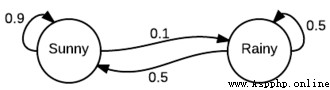
As you can see , It looks like a finite state machine , We just annotate the state transition with probability . for example , We can see if it's sunny today , The probability of sunny tomorrow is 0.9, The probability of rain is 0.1. It also starts on a rainy day . It should be clear that , From a given state , All outgoing conversions should total 1.0, Because it is a proper distribution .
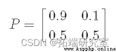
Another way to represent this information is through the transfer matrix P:
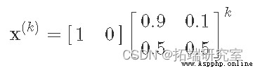
The interesting thing about expressing it as a matrix is , We can simulate Markov chains by matrix multiplication . for example , Suppose we start from a sunny state , We can express it as a row vector :x(0)=[10]. This implies that our probability of being in a sunny state is 1, So the probability of being in a rainy state is 0. Now? , If we perform matrix multiplication , We can find out the probability of being in each state after one step :
We can see that there will be 0.9 The chance of a sunny day ( According to our simple model ), Yes 0.1 The chance to rain . actually , We can continue to multiply the transformation matrix , In the k Step and find the sun / Opportunities for rain :
We can easily calculate x(k) Various k value , Use numpy:
import numpy as np
Pa = nps.ardraasy([[0.9, 0.1], [0.5, 0.5]])
istsdatea = np.arasdray([1, 0])
siasdmulatase_markasdov(istaasdte, P, 10)
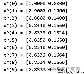
We can see an interesting phenomenon here , When we take more steps in the state machine , The probability of sunny or rainy days seems to converge . You may think this is related to our initial state , But it's not . If we initialize the initial state to a random value , We will get the same result :
siasmdulasteds_marksov(nap.arsdray([r, 1 - r]), P, 10)
x^(0) = [0.3653 0.6347]
x^(1) = [0.6461 0.3539]
x^(2) = [0.7584 0.2416]
x^(3) = [0.8034 0.1966]
x^(4) = [0.8214 0.1786]
x^(5) = [0.8285 0.1715]
x^(6) = [0.8314 0.1686]
x^(7) = [0.8326 0.1674]
x^(8) = [0.8330 0.1670]
x^(9) = [0.8332 0.1668]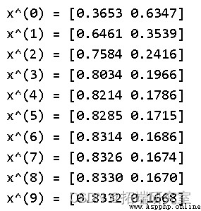
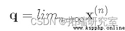
This steady-state distribution is called stationary distribution Usually use π Express . The steady state vector can be found in many ways π. The most direct way is in nn Take the limit when approaching infinity .
The next method is to solve the equation . Because by definition q It's steady state , So multiply by P Should return the same value :
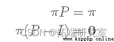
among I It's a unit matrix . If you extend our vector / Matrix symbol , You will find that this is just a set of equations and π1,π2,...,πn Sum to 1 ( namely π Form a probability distribution ). In our example, there are only two states :π1+π2=1.
However , Not every Markov chain has a stable distribution , Even the only one however , If we add two additional constraints to the Markov chain , We can guarantee these properties :
An important theorem says , If the Markov chain is ergodic , So it has a unique steady-state probability vector ππ. stay MCMC In the context of , We can jump from any state to any other state ( With a certain finite probability ), Easily satisfy irreducibility .
Another useful definition we will use is detailed balance and reversible Markov Chains. If there is a probability distribution that satisfies this condition π, Markov chains are said to be reversible ( Also known as detailed equilibrium conditions ):

let me put it another way , In the long run , You from the State i Move to state j The proportion of times , With you from the State j Move to state i The proportion of times is the same . in fact , If the Markov chain is reversible , Then we know that it has a stationary distribution ( That's why we use the same symbols π Why ).
Markov chain Monte Carlo (MCMC) The method is just a class of using Markov chains from a specific probability distribution ( Monte Carlo part ) Sampling algorithm in . They work by creating a Markov chain , Where the distribution is restricted ( Or smooth distribution ) It's just the distribution we want to sample .
This is a picture that may help to describe the process . Imagine , We are trying to make a MCMC To try to use PDF f(x) Sample any one-dimensional distribution . under these circumstances , Our state will be along x Point of axis , And our transition probability will be the opportunity to go from one state to another . This is a simplified diagram of the situation :
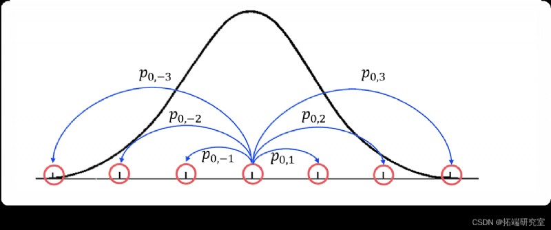
This figure shows the density function we are trying to approximate with a thick black line , And visualization of a part of a Markov chain using a blue line transiting from an orange state . especially , about i=-3,-2,-1,1,2,3, Just from the State X0 To Xi Transformation . however ,x Every point on the axis is actually a potential in this Markov chain . Please note that , That means we have an infinite state space , So we can no longer express the transformation well as a matrix .MCMC The real “ knack ” We want the design state ( or x The point on the axis ) Conversion probability between , So that we can spend most of our time f(x) In a large area , And there is relatively little time in its smaller area ( Is precisely proportional to our density function ).
As far as our characters are concerned , We want to spend most of our time around the center , Less time spent outside . in fact , If we simulate our Markov chain long enough , The restricted distribution of States should be similar to what we are trying to sample PDF. therefore , Use MCMC Method the basic algorithm for sampling is :
Now? , We are at every point x The proportional number of times spent on the axis should be what we are trying to simulate PDF Approximate value , That is, if we draw x Histogram of values , We should get the same shape .
Now? , Before we enter MCMC Method , I would like to introduce another method of sampling probability distribution , We'll use it later , be called rejection sampling. The main idea is , If we try to get from the distribution f(x) In the sample , We will use another tool to distribute g(x) To help from f(x) In the sample . The only limitation is for some M>1,f(x)<Mg(x). Its main use is when f(x) When it is difficult to sample directly ( But it can still be at any point xx Evaluate it ).
The following is a breakdown of the algorithm :
Another way to look at it is at our sampling point x0 Probability . This is the same as from g In the sample x0 Is proportional to the number of times we accept , It simply consists of f(x0) and Mg(x0) The ratio between :
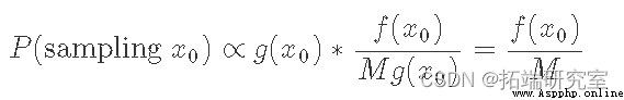
The equation tells us that the probability of sampling any point is equal to f(x0) In direct proportion to . After sampling many points and finding what we see x0 After the ratio of times , constant M Normalized , We got PDF f(x) The right result .
Let's take a more intuitive look at it through an example . The target distribution from which we want to sample f(x) yes double gamma Distribution , It's basically a two-sided gamma distribution . We will use the normal distribution g(x) As our envelope distribution . The following code shows us how to find the scaling constant M, It also describes how rejection sampling works conceptually .
# The goal is = Double gamma distribution
dsg = stats.dgamma(a=1)
# Generate PDF The sample of
x = np.linspace
# mapping
ax = df.plot(style=['--', '-'] 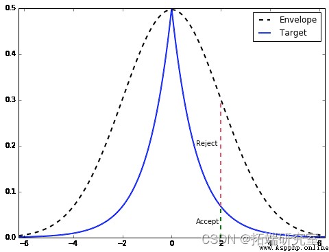
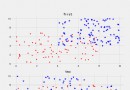
From the picture , Once we find g(x) The sample of ( under these circumstances x=2), We are equal to from the range Mg(x) Drawn in a uniform distribution of height . If it's on target PDF Within the height of , We accept it ( green ), Otherwise, refuse ( Refuse ).
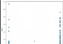
The following code implements reject sampling for our target dual gamma distribution . It draws standardized histograms and compares them with the theory we should get PDF matching .
# Generate samples from the reject sampling algorithm
sdampales = [rejeasdctioan_samplaing for x in range(10000)]
# Draw histogram and target PDF
df['Target'].plot
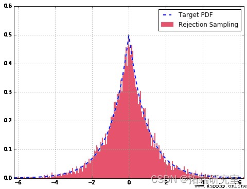
in general , Our reject sampler is very suitable for . Compared with the theoretical distribution , Taking more samples will improve the fitting .
A big part of reject sampling is that it's easy to implement ( stay Python Just a few lines of code ), But there is one major drawback : It's very slow .
this Metropolis-Hastings Algorithm (MH) It's a kind of MCMC technology , It extracts samples from probability distributions that are difficult to sample directly . Compared with refusal sampling , Yes MH The restrictions are actually more relaxed : For a given probability density function p(x), We only ask that we have one And p In direct proportion to Function of f(x)f(x) (x)p(x)! This is very useful when sampling posterior distributions .
In order to derive Metropolis-Hastings Algorithm , Let's start with the final goal : Create a Markov chain , Where the steady-state distribution is equal to our target distribution p(x). In terms of Markov chains , We already know what the state space will be : Support of probability distribution , namely x value . therefore ( Suppose the construction of Markov chain is correct ) The final steady-state distribution we get will be just p(x). The rest is to determine these x The probability of conversion between values , So that we can achieve this steady-state behavior .
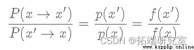
Detailed equilibrium conditions for Markov chains , Here it is written in another way :
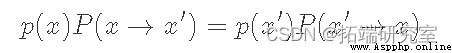
here p(x) Is our target distribution ,P(x→x′) From the point of x point-to-point x′ The probability of transfer . So our goal is to determine P(x→x′) In the form of . Since we want to build Markov chains , Let's start with equations 5 Start as the basis for this build . please remember , Detailed equilibrium conditions guarantee that our Markov chain will have a stable distribution ( It exists ). Besides , If we also include ergodicity ( Do not repeat the status at regular intervals , And each state can eventually reach any other state ), We will establish a unique stationary distribution p(x) The Markov chain of .
We can rearrange the equation to :
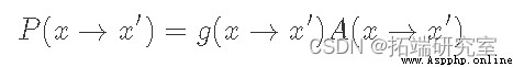
Here we use f(x) To represent a And p(x) A proportional function . This is to emphasize that we do not have a clear need p(x), It just needs something proportional to it , In this way, the ratio can achieve the same effect . Now here's “ skill ” Yes, we will P(x→x′) Break it down into two separate steps : A proposed distribution g(x→x′) And acceptance distribution A(x→x′)( Similar to the working principle of reject sampling ). Because they are independent , Our transition probability is just the product of the two :
here , We must find out g(x) and A(x) What is the right choice for . because g(x) yes “ Recommended distribution ”, It determines the next point we may sample . therefore , The important thing is that it has a distribution with our target p(x)( Ergodic condition ) Same support . A typical choice here is a normal distribution centered on the current state . Now let's give a fixed distribution of proposals g(x), We hope to find a match A(x).
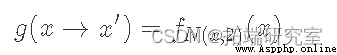
Although it's not obvious , But it satisfies the formula Of A(x) The typical choice is :
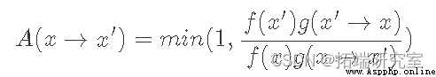
We can consider f(x′)g(x′→x) Less than or equal to 1 And greater than 1 The situation of . When less than or equal to 1 when , Its reciprocal is greater than 1, therefore LHS Denominator of ,A(x′→ x), equation 8 by 1, And the molecules are equal to RHS. perhaps , When f(x′)g(x′→x) It is greater than 1 LHS The molecule is 1, And the denominator happens to be RHS Reciprocal , Lead to LHS be equal to RHS.
such , We have proven that , The stable state of the Markov chain we create will be equal to our target distribution (p(x)), Because the detailed equilibrium conditions are satisfied by construction . So the overall algorithm will be ( With the above MCMC The algorithm matches very well ):
Before we move on , We need to discuss about MCMC Two very important topics of methods . The first topic relates to the initial state we chose . Because we randomly choose xx Value , It is likely to be located in p(x) A very small area ( Think about the tail of our double gamma distribution ). If you start here , It may take a disproportionate amount of time to traverse low-density x value , So as to give us a wrong feeling , That's all x Values should appear more frequently than they do . So the solution to this problem is “ Preburn ” The sampler generates a stack of samples and throws them away . The number of samples will depend on the details of the distribution we are trying to simulate .
The second problem we mentioned above is the correlation between two adjacent samples . Because according to our conversion function P(x→x′) The definition of , draw x′ Depending on the current state x. therefore , We have lost an important attribute of the sample : independence . To correct this , We extract Tth Samples , And only the last sample taken is recorded . hypothesis T Large enough , The sample should be relatively independent . Same as pre burning ,T The value of depends on the distribution of goals and proposals .
Let's use the double gamma distribution example above . Let's define our proposed distribution as x Centered 、 The standard deviation is 2、N(x, 2) Is a normal distribution ( remember x It's the current state ):
Given f(x) With our basic distribution p(x) Is proportional to the , Our acceptance distribution is as follows :
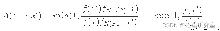
Because the normal distribution is symmetric , So normally distributed PDF They offset each other when evaluated at their respective points . Now let's look at some code :
# The simulation is proportional to the double gamma distribution f(x)
f = ambd x: g.df(x* mat.i
Sampler = mhspler()
# sample
sames = [nex(saper) for x in range(10000)]
# Draw histogram and target PDF
df['Target'].plot 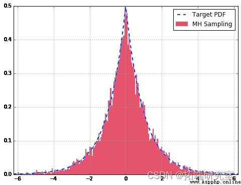
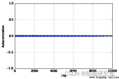
From us MH The sampler samples are well approximated to our double gamma distribution . Besides , View the autocorrelation diagram , We can see that it is very small in the whole sample , It shows that they are relatively independent . If we didn't do it for T Choose a good value or no pre burn period , We may see larger values in the graph .
I hope you enjoy this article about using refusal sampling and using Metropolis-Hastings Algorithm MCMC Sample short articles .

The most popular insights
1. Use R Language goes on METROPLIS-IN-GIBBS Sampling and MCMC function
2.R In language Stan Probabilistic programming MCMC Bayesian model of sampling
3.R Language implementation MCMC Medium Metropolis–Hastings Algorithm and Gibbs sampling
4.R Language BUGS JAGS Bayesian analysis Markov chain Monte Carlo method (MCMC) sampling
5.R In language block Gibbs Gibbs sampling Bayesian multiple linear regression
6.R Language Gibbs Bayesian simple linear regression simulation analysis of sampling
7.R Language use Rcpp Speed up Metropolis-Hastings Sample estimate the parameters of Bayesian logistic regression model
8.R Language use Metropolis- Hasting Sampling algorithm for logistic regression
9.R Sampling based on mixed data (MIDAS) Returning HAR-RV Model to predict GDP growth