above
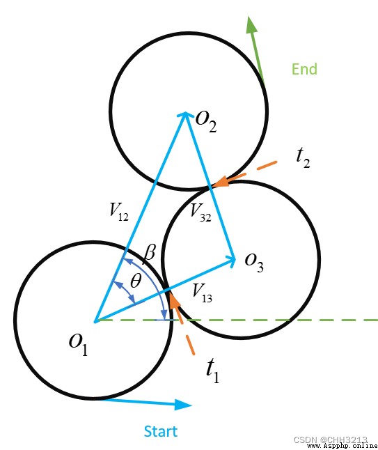
Dubins Curve derivation ( Vector based approach )
We have done this from the point of view of vector Dubins Derivation of curve formula , This blog is mainly based on this paper 《Classification of the Dubins set》 This paper introduces the relation based on geometry dubins The curve formula , Each case of the paper has a detailed derivation , So here is only the formula for each case , You can refer to the paper in the derivation process .
dubins The path set is { L S L , R S R , R S L , L S R , R L R , L R L } \{LSL, RSR, RSL, LSR, RLR, LRL\} { LSL,RSR,RSL,LSR,RLR,LRL}. L L L Represents a circular motion turning left , R R R Represents a right turning circular motion , S S S It means moving in a straight line .
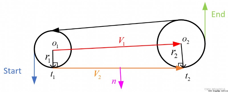
Set the starting point for s ( x i , y i , α i ) s\left(x_{i}, y_{i}, \alpha_{i}\right) s(xi,yi,αi) , The finish for g ( x g , y g , β g ) g\left(x_{g}, y_{g}, \beta_{g}\right) g(xg,yg,βg) , First, coordinate transformation will translate the starting point to the origin , And rotate θ \theta θ horn , Then the end will also fall x \mathrm{x} x On the shaft , The coordinates of the start and end points are s ( 0 , 0 , α ) , g ( d , 0 , β ) s(0,0, \alpha), g(d, 0, \beta) s(0,0,α),g(d,0,β) , among :
θ = atan 2 ( y g − y i x g − x i ) m o d { 2 π } D = ( x i − x g ) 2 + ( y i − y g ) 2 d = D / R α = ( α i − θ ) m o d { 2 π } β = ( β g − θ ) m o d { 2 π } (1) \tag{1} \begin{gathered} \theta=\operatorname{atan} 2\left(\frac{y_{g}-y_{i}}{x_{g}-x_{i}}\right) \bmod\{2\pi\} \\ D=\sqrt{\left(x_{i}-x_{g}\right)^{2}+\left(y_{i}-y_{g}\right)^{2}} \\ d=D / R \\ \alpha= \left(\alpha_{i}-\theta\right) \bmod\{2\pi\} \\ \beta= \left(\beta_{g}-\theta\right) \bmod\{2\pi\} \end{gathered} θ=atan2(xg−xiyg−yi)mod{ 2π}D=(xi−xg)2+(yi−yg)2d=D/Rα=(αi−θ)mod{ 2π}β=(βg−θ)mod{ 2π}(1)
Some notes :
among θ \theta θ Is the heading angle difference between the starting point and the terminal point , The angles above are [ 0 , 2 π ] [0,2 \pi] [0,2π] Between .
On it D D D Except for the above R R R This process can make each minimum turning radius R R R All for 1 , It is more convenient to calculate the arc length from the angle , The arc length is equal to the radian of the angle , So what you see later cos ( α ) \cos (\alpha) cos(α) , In fact, it is omitted from the front R R R .
m o d ( ) mod() mod() It's modular operation , for example : m o d ( 3 π , 2 π ) = 3 π m o d 2 π = π \bmod(3\pi,2\pi)=3\pi \bmod 2 \pi=\pi mod(3π,2π)=3πmod2π=π. The following β ( m o d 2 π ) \beta(\bmod 2 \pi) β(mod2π) That's what it means , namely β \beta β Yes 2 π 2\pi 2π modulus .python The implementation is simple , as follows :
def mod2pi(theta):
""" Yes 2pi Modulus operation """
return theta - 2.0 * math.pi * math.floor(theta / 2.0 / math.pi)
Coordinate transformation python It's easy to implement , as follows :
 # Coordinate transformation
dx = g_x-s_x
dy = g_y-s_y
D = math.hypot(dx, dy)
d = D * curvature
theta = mod2pi(math.atan2(dy, dx))
alpha = mod2pi(s_yaw - theta)
beta = mod2pi(g_yaw - theta)
Let the length of the vehicle on the starting circle be t t t , The length of straight-line segment is p p p , The length of the arc on the second circle is q q q, The entire path length L = t + p + q L=t+p+q L=t+p+q. The following are given in turn 6 The trajectory formula for two cases .
L S L LSL LSL The path length formula is as follows :
t l s l = − α + arctan cos β − cos α d + sin α − sin β { m o d 2 π } p l s l = 2 + d 2 − 2 cos ( α − β ) + 2 d ( sin α − sin β ) q l s l = β − arctan cos β − cos α d + sin α − sin β { m o d 2 π } (2) \tag{2} \begin{aligned} &t_{l s l}=-\alpha+\arctan \frac{\cos \beta-\cos \alpha}{d+\sin \alpha-\sin \beta}\{\bmod 2 \pi\} \\ &p_{l s l}=\sqrt{2+d^{2}-2 \cos (\alpha-\beta)+2 d(\sin \alpha-\sin \beta)} \\ &q_{l s l}=\beta-\arctan \frac{\cos \beta-\cos \alpha}{d+\sin \alpha-\sin \beta}\{\bmod 2 \pi\} \end{aligned} tlsl=−α+arctand+sinα−sinβcosβ−cosα{ mod2π}plsl=2+d2−2cos(α−β)+2d(sinα−sinβ)qlsl=β−arctand+sinα−sinβcosβ−cosα{ mod2π}(2)
The total length is equal to :
L l s l = t l s l + p l s l + q l s l = − α + β + p l s l (3) \tag{3} \mathcal{L}_{l s l}=t_{l s l}+p_{l s l}+q_{l s l}=-\alpha+\beta+p_{l s l} Llsl=tlsl+plsl+qlsl=−α+β+plsl(3)
python The implementation is as follows :
def left_straight_left(alpha, beta, d):
"""LSL route """
sa = math.sin(alpha)
sb = math.sin(beta)
ca = math.cos(alpha)
cb = math.cos(beta)
c_ab = math.cos(alpha - beta)
tmp0 = d + sa - sb
mode = ["L", "S", "L"]
p_squared = 2 + (d * d) - (2 * c_ab) + (2 * d * (sa - sb))
if p_squared < 0:
return None, None, None, mode
tmp1 = math.atan2((cb - ca), tmp0)
t = mod2pi(-alpha + tmp1)
p = math.sqrt(p_squared)
q = mod2pi(beta - tmp1)
return t, p, q, mode
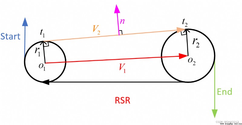
R S R RSR RSR The path length formula is as follows :
t r s r = α − arctan cos α − cos β d − sin α + sin β { m o d 2 π } p r s r = 2 + d 2 − 2 cos ( α − β ) + 2 d ( sin β − sin α ) q r s r = − β ( m o d 2 π ) + arctan cos α − cos β d − sin α + sin β { m o d 2 π } (4) \tag{4} \begin{aligned} t_{r s r} &=\alpha-\arctan \frac{\cos \alpha-\cos \beta}{d-\sin \alpha+\sin \beta}\{\bmod 2 \pi\} \\ p_{r s r} &=\sqrt{2+d^{2}-2 \cos (\alpha-\beta)+2 d(\sin \beta-\sin \alpha)} \\ q_{r s r} &=-\beta(\bmod 2 \pi)+\arctan \frac{\cos \alpha-\cos \beta}{d-\sin \alpha+\sin \beta}\{\bmod 2 \pi\} \\ \end{aligned} trsrprsrqrsr=α−arctand−sinα+sinβcosα−cosβ{ mod2π}=2+d2−2cos(α−β)+2d(sinβ−sinα)=−β(mod2π)+arctand−sinα+sinβcosα−cosβ{ mod2π}(4)
The total length is equal to :
L r s r = t r s r + p r s r + q r s r = α − β + p r s r (5) \tag{5} \mathcal{L}_{r s r} =t_{r s r}+p_{r s r}+q_{r s r}=\alpha-\beta+p_{r s r} Lrsr=trsr+prsr+qrsr=α−β+prsr(5)
python The implementation is as follows :
def right_straight_right(alpha, beta, d):
"""RSR route """
sa = math.sin(alpha)
sb = math.sin(beta)
ca = math.cos(alpha)
cb = math.cos(beta)
c_ab = math.cos(alpha - beta)
tmp0 = d - sa + sb
mode = ["R", "S", "R"]
p_squared = 2 + (d * d) - (2 * c_ab) + (2 * d * (sb - sa))
if p_squared < 0:
return None, None, None, mode
tmp1 = math.atan2((ca - cb), tmp0)
t = mod2pi(alpha - tmp1)
p = math.sqrt(p_squared)
q = mod2pi(-mod2pi(beta) + tmp1)
return t, p, q, mode
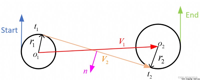
R S L RSL RSL The path length formula is as follows :
t r s l = α − arctan ( cos α + cos β d − sin α − sin β ) + arctan ( 2 p r s l ) { m o d 2 π } p r s l = d 2 − 2 + 2 cos ( α − β ) − 2 d ( sin α + sin β ) q r s l = β ( m o d 2 π ) − arctan ( cos α + cos β d − sin α − sin β ) + arctan ( 2 p r s l ) { m o d 2 π } (6) \tag{6} \begin{aligned} t_{r s l} &=\alpha-\arctan \left(\frac{\cos \alpha+\cos \beta}{d-\sin \alpha-\sin \beta}\right)+\arctan \left(\frac{2}{p_{r s l}}\right)\{\bmod 2 \pi\} \\ p_{r s l} &=\sqrt{d^{2}-2+2 \cos (\alpha-\beta)-2 d(\sin \alpha+\sin \beta)} \\ q_{r s l} &=\beta(\bmod 2 \pi)-\arctan \left(\frac{\cos \alpha+\cos \beta}{d-\sin \alpha-\sin \beta}\right)+\arctan \left(\frac{2}{p_{r s l}}\right)\{\bmod 2 \pi\} \\ \end{aligned} trslprslqrsl=α−arctan(d−sinα−sinβcosα+cosβ)+arctan(prsl2){ mod2π}=d2−2+2cos(α−β)−2d(sinα+sinβ)=β(mod2π)−arctan(d−sinα−sinβcosα+cosβ)+arctan(prsl2){ mod2π}(6)
The total length is equal to :
L r s l = t r s l + p r s l + q r s l = − α + β + 2 t r s l + p r s l (7) \tag{7} \mathcal{L}_{r s l} =t_{r s l}+p_{r s l}+q_{r s l}=-\alpha+\beta+2 t_{r s l}+p_{r s l} Lrsl=trsl+prsl+qrsl=−α+β+2trsl+prsl(7)
python The implementation is as follows :
def right_straight_left(alpha, beta, d):
"""RSL route """
sa = math.sin(alpha)
sb = math.sin(beta)
ca = math.cos(alpha)
cb = math.cos(beta)
c_ab = math.cos(alpha - beta)
p_squared = (d * d) - 2 + (2 * c_ab) - (2 * d * (sa + sb))
mode = ["R", "S", "L"]
if p_squared < 0:
return None, None, None, mode
p = math.sqrt(p_squared)
tmp2 = math.atan2((ca + cb), (d - sa - sb)) - math.atan2(2.0, p)
t = mod2pi(alpha - tmp2)
q = mod2pi(mod2pi(beta) - tmp2)
return t, p, q, mode
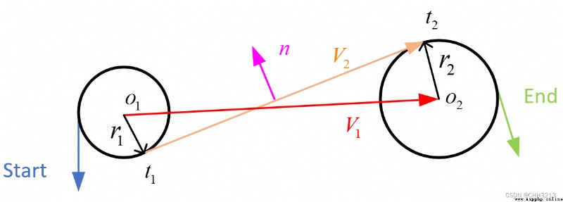
L S R LSR LSR The path length formula is as follows :
t l s r = ( − α + arctan ( − cos α − cos β d + sin α + sin β ) − arctan ( − 2 p l s r ) ) { m o d 2 π } p l s r = − 2 + d 2 + 2 cos ( α − β ) + 2 d ( sin α + sin β ) q l s r = − β ( m o d 2 π ) + arctan ( − cos α − cos β d + sin α + sin β ) − arctan ( − 2 p l s r ) { m o d 2 π } (8) \tag{8} \begin{aligned} t_{l s r} &=\left(-\alpha+\arctan \left(\frac{-\cos \alpha-\cos \beta}{d+\sin \alpha+\sin \beta}\right)-\arctan \left(\frac{-2}{p_{l s r}}\right)\right)\{\bmod 2 \pi\} \\ p_{l s r} &=\sqrt{-2+d^{2}+2 \cos (\alpha-\beta)+2 d(\sin \alpha+\sin \beta)} \\ q_{l s r} &=-\beta(\bmod 2 \pi)+\arctan \left(\frac{-\cos \alpha-\cos \beta}{d+\sin \alpha+\sin \beta}\right)-\arctan \left(\frac{-2}{p_{l s r}}\right)\{\bmod 2 \pi\} \\ \end{aligned} tlsrplsrqlsr=(−α+arctan(d+sinα+sinβ−cosα−cosβ)−arctan(plsr−2)){ mod2π}=−2+d2+2cos(α−β)+2d(sinα+sinβ)=−β(mod2π)+arctan(d+sinα+sinβ−cosα−cosβ)−arctan(plsr−2){ mod2π}(8)
The total length is equal to :
L l s r = t l s r + p l s r + q l s r = α − β + 2 t l s r + p l s r (9) \tag{9} \mathcal{L}_{l s r} =t_{l s r}+p_{l s r}+q_{l s r}=\alpha-\beta+2 t_{l s r}+p_{l s r} Llsr=tlsr+plsr+qlsr=α−β+2tlsr+plsr(9)
python The implementation is as follows :
def left_straight_right(alpha, beta, d):
"""LSR route """
sa = math.sin(alpha)
sb = math.sin(beta)
ca = math.cos(alpha)
cb = math.cos(beta)
c_ab = math.cos(alpha - beta)
p_squared = -2 + (d * d) + (2 * c_ab) + (2 * d * (sa + sb))
mode = ["L", "S", "R"]
if p_squared < 0:
return None, None, None, mode
p = math.sqrt(p_squared)
tmp2 = math.atan2((-ca - cb), (d + sa + sb)) - math.atan2(-2.0, p)
t = mod2pi(-alpha + tmp2)
q = mod2pi(-mod2pi(beta) + tmp2)
return t, p, q, mode
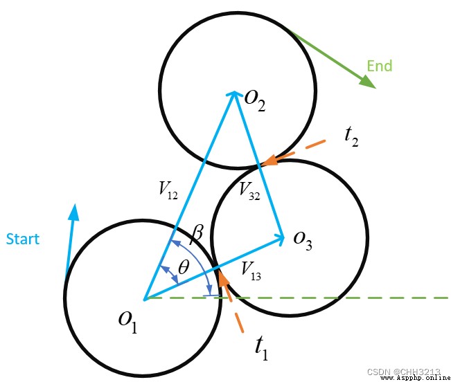
R L R RLR RLR The path length formula is as follows :
t r l r = α − arctan ( cos α − cos β d − sin α + sin β ) + p r l r 2 { m o d 2 π } p r l r = arccos 1 8 ( 6 − d 2 + 2 cos ( α − β ) + 2 d ( sin α − sin β ) ) q r l r = α − β − t r l r + p r l r { m o d 2 π } (10) \tag{10} \begin{aligned} &t_{r l r}=\alpha-\arctan \left(\frac{\cos \alpha-\cos \beta}{d-\sin \alpha+\sin \beta}\right)+\frac{p_{r l r}}{2}\{\bmod 2 \pi\} \\ &p_{r l r}=\arccos \frac{1}{8}\left(6-d^{2}+2 \cos (\alpha-\beta)+2 d(\sin \alpha-\sin \beta)\right) \\ &q_{r l r}=\alpha-\beta-t_{r l r}+p_{r l r}\{\bmod 2 \pi\} \\ \end{aligned} trlr=α−arctan(d−sinα+sinβcosα−cosβ)+2prlr{ mod2π}prlr=arccos81(6−d2+2cos(α−β)+2d(sinα−sinβ))qrlr=α−β−trlr+prlr{ mod2π}(10)
The total length is equal to :
L r l r = t r l r + p r l r + q r l r = α − β + 2 p r l r (11) \tag{11} \mathcal{L}_{r l r}=t_{r l r}+p_{r l r}+q_{r l r}=\alpha-\beta+2 p_{r l r} Lrlr=trlr+prlr+qrlr=α−β+2prlr(11)
python The implementation is as follows :
def right_left_right(alpha, beta, d):
"""RLR route """
sa = math.sin(alpha)
sb = math.sin(beta)
ca = math.cos(alpha)
cb = math.cos(beta)
c_ab = math.cos(alpha - beta)
mode = ["R", "L", "R"]
tmp_rlr = (6.0 - d * d + 2.0 * c_ab + 2.0 * d * (sa - sb)) / 8.0
if abs(tmp_rlr) > 1.0:
return None, None, None, mode
p = mod2pi(math.acos(tmp_rlr))
t = mod2pi(alpha - math.atan2(ca - cb, d - sa + sb) + mod2pi(p / 2.0))
q = mod2pi(alpha - beta - t + p)
return t, p, q, mode
The above implementation method can not get the optimal result , It's strange , The best result can be obtained by the following method :
def right_left_right(alpha, beta, d):
"""RLR route , The implementation of this part is inconsistent with the formula , If it is changed to be consistent with the formula, the optimal path will not be obtained """
sa = math.sin(alpha)
sb = math.sin(beta)
ca = math.cos(alpha)
cb = math.cos(beta)
c_ab = math.cos(alpha - beta)
mode = ["R", "L", "R"]
tmp_rlr = (6.0 - d * d + 2.0 * c_ab + 2.0 * d * (sa - sb)) / 8.0
if abs(tmp_rlr) > 1.0:
return None, None, None, mode
p = mod2pi(2 * math.pi - math.acos(tmp_rlr))
t = mod2pi(alpha - math.atan2(ca - cb, d - sa + sb) + mod2pi(p / 2.0))
q = mod2pi(alpha - beta - t + mod2pi(p))
return t, p, q, mode
L R L LRL LRL The path length formula is as follows :
t l r l = ( − α + arctan ( − cos α + cos α d + sin α − sin β ) + p l r l 2 ) { m o d 2 π } p l r l = arccos 1 8 ( 6 − d 2 + 2 cos ( α − β ) + 2 d ( sin α − sin β ) ) { m o d 2 π } q l r l = β ( m o d 2 π ) − α + 2 p l r l { m o d 2 π } (12) \tag{12} \begin{aligned} &t_{l r l}=\left(-\alpha+\arctan \left(\frac{-\cos \alpha+\cos \alpha}{d+\sin \alpha-\sin \beta}\right)+\frac{p_{l r l}}{2}\right)\{\bmod 2 \pi\} \\ &p_{l r l}=\arccos \frac{1}{8}\left(6-d^{2}+2 \cos (\alpha-\beta)+2 d(\sin \alpha-\sin \beta)\right)\{\bmod 2 \pi\} \\ &q_{l r l}=\beta(\bmod 2 \pi)-\alpha+2 p_{l r l}\{\bmod 2 \pi\} \end{aligned} tlrl=(−α+arctan(d+sinα−sinβ−cosα+cosα)+2plrl){ mod2π}plrl=arccos81(6−d2+2cos(α−β)+2d(sinα−sinβ)){ mod2π}qlrl=β(mod2π)−α+2plrl{ mod2π}(12)
The total length is equal to :
L l r l = t l r l + p l r l + q l r l = − α + β + 2 p l r l . (13) \tag{13} \mathcal{L}_{l r l}=t_{l r l}+p_{l r l}+q_{l r l}=-\alpha+\beta+2 p_{l r l} . Llrl=tlrl+plrl+qlrl=−α+β+2plrl.(13)
python The implementation is as follows :
def left_right_left(alpha, beta, d):
"""LRL route """
sa = math.sin(alpha)
sb = math.sin(beta)
ca = math.cos(alpha)
cb = math.cos(beta)
c_ab = math.cos(alpha - beta)
mode = ["L", "R", "L"]
tmp_lrl = (6.0 - d * d + 2.0 * c_ab + 2.0 * d * (- sa + sb)) / 8.0
if abs(tmp_lrl) > 1:
return None, None, None, mode
p = mod2pi(math.acos(tmp_lrl))
t = mod2pi(-alpha - math.atan2(ca - cb, d + sa - sb) + p / 2.0)
q = mod2pi(mod2pi(beta) - alpha +2*p)
return t, p, q, mode
Similarly, the above implementation method can not get the optimal result , The best result can be obtained by the following method :
def left_right_left(alpha, beta, d):
"""LRL route , The implementation of this part is inconsistent with the formula , If it is changed to be consistent with the formula, the optimal path will not be obtained """
sa = math.sin(alpha)
sb = math.sin(beta)
ca = math.cos(alpha)
cb = math.cos(beta)
c_ab = math.cos(alpha - beta)
mode = ["L", "R", "L"]
tmp_lrl = (6.0 - d * d + 2.0 * c_ab + 2.0 * d * (- sa + sb)) / 8.0
if abs(tmp_lrl) > 1:
return None, None, None, mode
p = mod2pi(2 * math.pi - math.acos(tmp_lrl))
t = mod2pi(-alpha - math.atan2(ca - cb, d + sa - sb) + p / 2.0)
q = mod2pi(mod2pi(beta) - alpha - t + mod2pi(p))
return t, p, q, mode
For the complete code file above, see github Warehouse