PCAThe algorithm is a principal component analysis algorithm,found in the dataset“主成分”,Can be used to compress data dimensions.
We'll go through one first2D數據集進行實驗,以獲得關於PCA如何工作的直觀感受,然後在一個更大的圖像數據集上使用它.
PCA算法的好處如下:
1.使得數據集更易使用
2.降低算法的計算開銷
3.去除噪聲
4.使得結果更易理解
Linear regression and neural network algorithms,can be used firstPCA對數據進行降維.
關於PCAThe theoretical part of the algorithm,可以參考我之前的博客:
https://blog.csdn.net/wzk4869/article/details/126017831?spm=1001.2014.3001.5501
老樣子,Put the dataset you want to use first:
鏈接:https://pan.baidu.com/s/1_8yJo58oCuuo6ZasaC5R3A
提取碼:6666
導入需要的包
import matplotlib.pyplot as plt
import matplotlib as mpl
from scipy.io import loadmat
from numpy import *
import pandas as pd
導入數據集
def load_dataset():
path='./data/ex7data1.mat'
two_dimension_data=loadmat(path)
X=two_dimension_data['X']
return X
Let's take a look at the corresponding dataset:
[[3.38156267 3.38911268]
[4.52787538 5.8541781 ]
[2.65568187 4.41199472]
[2.76523467 3.71541365]
[2.84656011 4.17550645]
[3.89067196 6.48838087]
[3.47580524 3.63284876]
[5.91129845 6.68076853]
[3.92889397 5.09844661]
[4.56183537 5.62329929]
[4.57407171 5.39765069]
[4.37173356 5.46116549]
[4.19169388 4.95469359]
[5.24408518 4.66148767]
[2.8358402 3.76801716]
[5.63526969 6.31211438]
[4.68632968 5.6652411 ]
[2.85051337 4.62645627]
[5.1101573 7.36319662]
[5.18256377 4.64650909]
[5.70732809 6.68103995]
[3.57968458 4.80278074]
[5.63937773 6.12043594]
[4.26346851 4.68942896]
[2.53651693 3.88449078]
[3.22382902 4.94255585]
[4.92948801 5.95501971]
[5.79295774 5.10839305]
[2.81684824 4.81895769]
[3.88882414 5.10036564]
[3.34323419 5.89301345]
[5.87973414 5.52141664]
[3.10391912 3.85710242]
[5.33150572 4.68074235]
[3.37542687 4.56537852]
[4.77667888 6.25435039]
[2.6757463 3.73096988]
[5.50027665 5.67948113]
[1.79709714 3.24753885]
[4.3225147 5.11110472]
[4.42100445 6.02563978]
[3.17929886 4.43686032]
[3.03354125 3.97879278]
[4.6093482 5.879792 ]
[2.96378859 3.30024835]
[3.97176248 5.40773735]
[1.18023321 2.87869409]
[1.91895045 5.07107848]
[3.95524687 4.5053271 ]
[5.11795499 6.08507386]]
(50, 2)
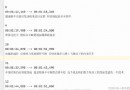
繪制散點圖
def plot_scatter(X):
plt.figure(figsize=(12,8))
plt.scatter(X[:,0],X[:,1])
plt.show()
Let's take a look at the scatterplot after visualization:
去均值化
The result we return is the de-averaged data,並生成散點圖:
def demean(X):
X_demean=(X-mean(X,axis=0))
plt.figure(figsize=(12,8))
plt.scatter(X_demean[:,0],X_demean[:,1])
plt.show()
return X_demean

計算數據的協方差矩陣
def sigma_matrix(X_demean):
sigma=(X_demean.T @ X_demean)/X_demean.shape[0]
return sigma
[[1.34852518 0.86535019]
[0.86535019 1.02641621]]
計算特征值、特征向量
def usv(sigma):
u,s,v=linalg.svd(sigma)
return u,s,v
[[-0.76908153 -0.63915068]
[-0.63915068 0.76908153]]
====================================================================================================
[2.06768062 0.30726078]
====================================================================================================
[[-0.76908153 -0.63915068]
[-0.63915068 0.76908153]]
對數據進行降維
對數據進行降維,降維後得到Z,在二維數據中ZThe data is a line of points(一維).
def project_data(X_demean, u, k):
u_reduced = u[:,:k]
z=dot(X_demean, u_reduced)
return z
[[ 1.49876595]
[-0.95839024]
[ 1.40325172]
[ 1.76421694]
[ 1.40760243]
[-0.87367998]
[ 1.27050164]
[-2.5506712 ]
[-0.01469839]
[-0.83694188]
[-0.70212917]
[-0.58711016]
[-0.12493311]
[-0.74690506]
[ 1.67629396]
[-2.10275704]
[-0.9594953 ]
[ 1.11633715]
[-2.37070273]
[-0.69001651]
[-2.39397485]
[ 0.44284714]
[-1.98340505]
[-0.01058959]
[ 1.83205377]
[ 0.62719172]
[-1.33171608]
[-1.4546727 ]
[ 1.01919098]
[ 0.01489202]
[-0.07212622]
[-1.78539513]
[ 1.41318051]
[-0.82644523]
[ 0.75167377]
[-1.40551081]
[ 1.82309802]
[-1.59458841]
[ 2.80783613]
[-0.32551527]
[-0.98578762]
[ 0.98465469]
[ 1.38952836]
[-1.03742062]
[ 1.87686597]
[-0.24535117]
[ 3.51800218]
[ 1.54860441]
[ 0.34412682]
[-1.55978675]]
還原數據
def recover_data(z, u, k):
u_reduced = u[:,:k]
X_recover=dot(z, u_reduced.T)
return X_recover
[[-1.15267321 -0.95793728]
[ 0.73708023 0.61255577]
[-1.07921498 -0.89688929]
[-1.35682667 -1.12760046]
[-1.08256103 -0.89967005]
[ 0.67193114 0.55841316]
[-0.97711935 -0.81204199]
[ 1.96167412 1.63026324]
[ 0.01130426 0.00939449]
[ 0.64367655 0.53493198]
[ 0.53999458 0.44876634]
[ 0.45153559 0.37525186]
[ 0.09608375 0.07985108]
[ 0.57443089 0.47738488]
[-1.28920673 -1.07140443]
[ 1.61719161 1.34397859]
[ 0.73793012 0.61326208]
[-0.85855429 -0.71350765]
[ 1.82326369 1.51523626]
[ 0.53067896 0.44102452]
[ 1.84116185 1.53011066]
[-0.34058556 -0.28304605]
[ 1.5254002 1.26769469]
[ 0.00814426 0.00676834]
[-1.40899873 -1.17095842]
[-0.48236157 -0.40087002]
[ 1.02419824 0.85116724]
[ 1.11876191 0.92975505]
[-0.78384096 -0.65141661]
[-0.01145318 -0.00951825]
[ 0.05547094 0.04609952]
[ 1.37311442 1.14113651]
[-1.08685103 -0.90323529]
[ 0.63560376 0.52822303]
[-0.57809841 -0.4804328 ]
[ 1.08095241 0.89833319]
[-1.40211102 -1.16523434]
[ 1.2263685 1.01918227]
[-2.15945492 -1.79463038]
[ 0.25034779 0.20805331]
[ 0.75815106 0.63006683]
[-0.75727974 -0.62934272]
[-1.0686606 -0.888118 ]
[ 0.79786104 0.6630681 ]
[-1.44346296 -1.19960017]
[ 0.18869505 0.15681637]
[-2.70563051 -2.24853349]
[-1.19100306 -0.98979157]
[-0.26466158 -0.21994889]
[ 1.19960319 0.99693877]]
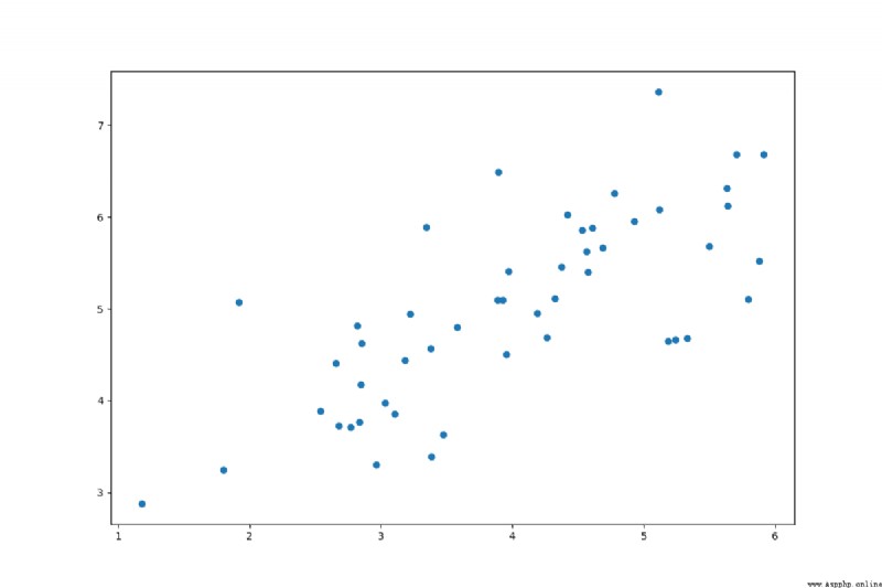
數據可視化
fig, ax = plt.subplots(figsize=(12, 8))
ax.scatter(X_demean[:,0],X_demean[:,1])
ax.scatter(list(X_recover[:, 0]), list(X_recover[:, 1]),c='r')
ax.plot([X_demean[:,0],list(X_recover[:, 0])],[X_demean[:,1],list(X_recover[:, 1])])
plt.show()
import matplotlib.pyplot as plt
import matplotlib as mpl
from scipy.io import loadmat
from numpy import *
import pandas as pd
""" PCADimensionality reduction for two-dimensional data """
def load_dataset():
path='./data/ex7data1.mat'
two_dimension_data=loadmat(path)
X=two_dimension_data['X']
return X
def plot_scatter(X):
plt.figure(figsize=(12,8))
cm=mpl.colors.ListedColormap(['blue'])
plt.scatter(X[:,0],X[:,1],cmap=cm)
plt.show()
""" 對X去均值,並可視化圖像 """
def demean(X):
X_demean=(X-mean(X,axis=0))
plt.figure(figsize=(12,8))
plt.scatter(X_demean[:,0],X_demean[:,1])
plt.show()
return X_demean
""" 計算協方差矩陣 """
def sigma_matrix(X_demean):
sigma=(X_demean.T @ X_demean)/X_demean.shape[0]
return sigma
""" 計算特征值、特征向量 """
def usv(sigma):
u,s,v=linalg.svd(sigma)
return u,s,v
def project_data(X_demean, u, k):
u_reduced = u[:,:k]
z=dot(X_demean, u_reduced)
return z
def recover_data(z, u, k):
u_reduced = u[:,:k]
X_recover=dot(z, u_reduced.T)
return X_recover
if __name__=='__main__':
X=load_dataset()
print(X)
print('=='*50)
print(X.shape)
print('=='*50)
plot_scatter(X)
X_demean=demean(X)
sigma=sigma_matrix(X_demean)
print(sigma)
print('=='*50)
u, s, v=usv(sigma)
print(u)
print('=='*50)
print(s)
print('=='*50)
print(v)
print('=='*50)
z = project_data(X_demean, u, 1)
print(z)
print('=='*50)
X_recover = recover_data(z, u, 1)
print(X_recover)
print('=='*50)
fig, ax = plt.subplots(figsize=(12, 8))
ax.scatter(X_demean[:,0],X_demean[:,1])
ax.scatter(list(X_recover[:, 0]), list(X_recover[:, 1]),c='r')
ax.plot([X_demean[:,0],list(X_recover[:, 0])],[X_demean[:,1],list(X_recover[:, 1])])
plt.show()