This article “python OpenCV Example analysis of image pyramid ” Most people don't quite understand the knowledge points of the article , So I made up the following summary for you , Detailed content , The steps are clear , It has certain reference value , I hope you can gain something after reading this article , Let's take a look at this article “python OpenCV Example analysis of image pyramid ” Article bar .
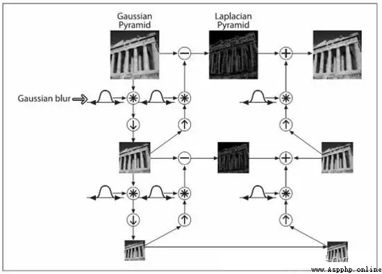
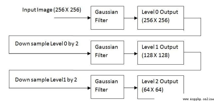
Image pyramid is a kind of multi-scale expression of image , It is an effective but simple concept structure for interpreting images at multi-resolution . The pyramid of an image is a series of pyramid shaped pyramids with gradually decreasing resolution , And from the same original image set . It is obtained by step down sampling , Stop sampling until a certain termination condition is reached . We compare layers of images to pyramids , The higher the level , The smaller the image , Lower resolution .
Then why should we make an image pyramid ? This is because changing the pixel size sometimes does not change its characteristics , Let's show you 1000 Megapixel image , You know there's someone inside , I'll show you a 100000 pixel , You can also know there's someone inside , But for computers , Processing 100000 pixels, comparable processing 1000 Ten thousand pixels is much easier . To make it easier for computers to recognize features , Later, we will also talk about the practical project of feature recognition , Maybe you played basketball in high school , I saw your head teacher coming out from afar , You leave 500 rice , You can still recognize your teachers by their characteristics , Leave you with your head teacher 2 It's the same with rice .
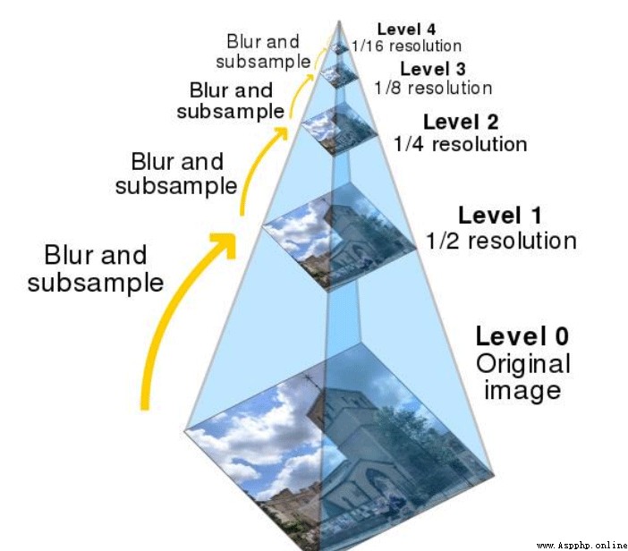
in other words Image pyramid a collection of subgraphs with different resolutions of the same image . Here we can give an example that the original image is a 400400 Image , Then take it up and it will be 200200 And then 100*100, This reduces the resolution , But it's always the same image .
So from the first i Layer to tier i+1 layer , How exactly did he do it ?
1. Calculate the approximate value of the reduced resolution of the input image . This can be done by filtering the input and 2 Sample for step size ( Subsampling ). There are many filtering operations that can be used , Such as neighborhood average ( The average pyramid can be generated ), Gaussian low pass filter ( Gaussian pyramid can be generated ), Or no filtering , Generate sub sampling pyramid . The quality of the generated approximation is a function of the selected filter . No filter , The confusion in the upper layer of the pyramid becomes obvious , The sub sampling points are not very representative of the selected area .
2. Interpolate the output from the previous step ( The factor is still 2) And filter it . This will generate a predictive image with the same resolution as the input . Because in step 1 Interpolation between the output pixels of , So the insertion filter determines the predicted value and the steps 1 The degree of approximation between the inputs of . If the insertion filter is ignored , Then the predicted value will be step 1 Interpolation form of output , The block effect of duplicate pixels will become obvious .
3. computational procedure 2 The predicted values and steps 1 The difference between the inputs of . With j The difference identified by the level prediction residual will be used for the reconstruction of the original image . Without quantifying the difference , The prediction residual pyramid can be used to generate the corresponding approximate pyramid ( Including the original image ), Without error .
Perform the above process P Times will produce closely related P+1 First order approximation and prediction residual pyramid .j-1 The output of the first approximation is used to provide an approximation pyramid , and j The output of level prediction residuals is placed in the prediction residuals pyramid . If you don't need a prediction residual pyramid , Then step 2 and 3、 Interpolator 、 The insertion filter and the adder in the figure can be omitted .
Here, down sampling represents the reduction of the image . Upsampling indicates an increase in image size .
1. To image Gi Gaussian kernel convolution .
Gaussian kernel convolution is what we call Gaussian filter manipulation , We have already talked about , Use a Gaussian convolution kernel , Let the adjacent pixel value take a larger weight , Then do relevant operations with the target image .
2. Delete all even rows and columns .
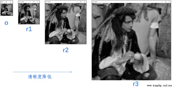
original image M * N Processing results M/2 * N/2. After each treatment , The resulting image is the original 1/4. This operation is called Octave. Repeat the process , Construct image pyramids . Until the image can not be further divided . This process will lose image information .
Sampling upward is just the opposite of sampling downward , On the original image ,** Expand into the original in each direction 2 times , New rows and columns with 0 fill . Use with “ Use... Downward ” The same convolution kernel times 4, obtain “ New pixels ” The new value of .** The image will be blurred after upward sampling .
Sampling up 、 Down sampling is not an inverse operation . After two operations , Unable to restore the original image .
Image pyramid down sampling function :
dst=cv2.pyrDown(src)
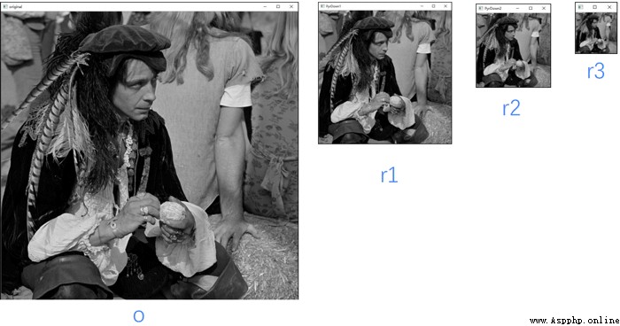
import cv2import numpy as npo=cv2.imread("image\\man.bmp")r1=cv2.pyrDown(o)r2=cv2.pyrDown(r1)r3=cv2.pyrDown(r2)cv2.imshow("original",o)cv2.imshow("PyrDown1",r1)cv2.imshow("PyrDown2",r2)cv2.imshow("PyrDown3",r3)cv2.waitKey()cv2.destroyAllWindows()Here we do three down sampling on the image , The result is :
Down sampling will lose information !!!
Image pyramid up sampling function :
dst=cv2.pyrUp(src)
We won't introduce the code here .
Take a look at our results directly :
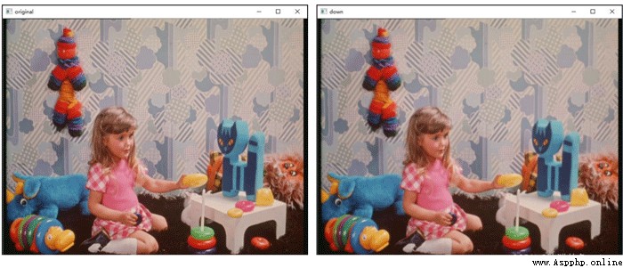
Here, let's take a look at the image after sampling downward and then sampling upward , Is it consistent . There is also the image sampling upward and then downward , Are they consistent ? Here we do some research with the image of a little girl .
First of all, let's analyze it : When the image is sampled down once , Image by MN Turned into M/2N/2, Then, after upward sampling again, it becomes M*N. So it can be proved that for the picture size It doesn't change .
import cv2o=cv2.imread("image\\girl.bmp")down=cv2.pyrDown(o)up=cv2.pyrUp(down)cv2.imshow("original",o)cv2.imshow("down",down)cv2.imshow("up",up)cv2.waitKey()cv2.destroyAllWindows()So let's see what has changed ?
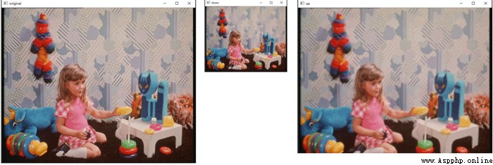
It can be clearly seen here that the picture of the little girl has become blurred , So why ? Because as we mentioned above, when the image becomes smaller , Then you will lose some information , After zooming in again , Because the convolution kernel gets bigger , Then the image will become blurred . So it will not be consistent with the original image .
Then let's take a look at the upward sampling operation first , What would it look like to do a downward sampling operation ? Since the image becomes too large, we omit the image sampled upward from the intermediate image .
Then it is not particularly easy for us to find differences with the naked eye , So let's use image subtraction to see .
import cv2o=cv2.imread("image\\girl.bmp")up=cv2.pyrUp(o)down=cv2.pyrDown(up)diff=down-o # structure diff Images , see down And o The difference between cv2.imshow("difference",diff)cv2.waitKey()cv2.destroyAllWindows()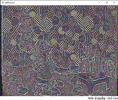
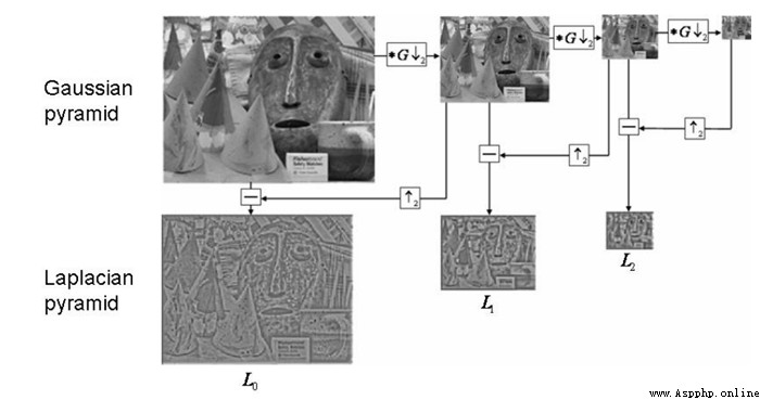
Let's first look at what the Laplace pyramid is :
Li = Gi - PyrUp(PyrDown(Gi))
We can know from his formula , Laplacian pyramid is a process of subtracting downward sampling from the original image and then upward sampling .
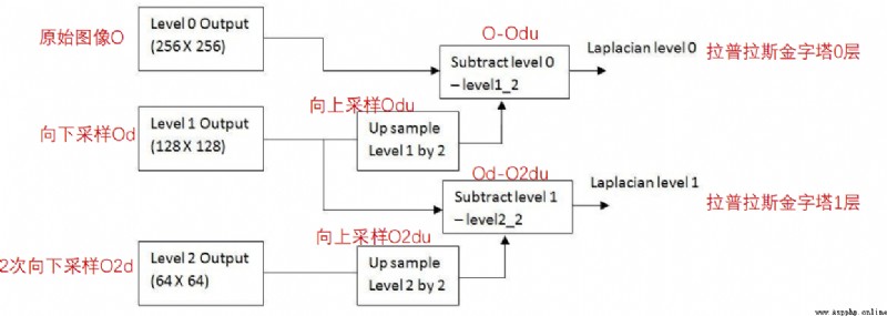
Displayed in the image is :
The core function is :
od=cv2.pyrDown(o)odu=cv2.pyrUp(od)lapPyr=o-odu
First of all, we need to explain that the contour of the image is different from the edge of the image , The edges are scattered , But the outline is a whole .
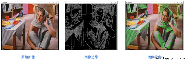
Edge detection can detect edges , But the edges are discontinuous . Connect the edges as a whole , Form an outline .
Be careful :
The object is a binary image . Therefore, it is necessary to perform threshold segmentation or edge detection in advance . Finding the contour requires changing the original image . therefore , Usually a copy of the original image is used . stay OpenCV in , Is to find white objects from a black background . therefore , The object must be white , The background must be black .
For the detection of image contour, the required function is :
cv2.findContours( ) and cv2.drawContours( )
The function to find the image outline is cv2.findContours(), adopt cv2.drawContours() Draw the found contour onto the image .
about cv2.findContours( ) function :
image, contours, hierarchy = cv2.findContours( image, mode, method)
Note here that in the latest version , There are only two return functions in the contour :
contours, hierarchy = cv2.findContours( image, mode, method)
contours , outline
hierarchy , The topological information of the image ( Contour hierarchy )
image , original image
mode , Contour retrieval mode
method , The approximate method of contour
Here we need to introduce mode: That is, contour retrieval mode :
cv2.RETR_EXTERNAL : Indicates that only the outer contour is detected
cv2.RETR_LIST : The detected contour does not establish a hierarchical relationship
cv2.RETR_CCOMP : Build two levels of outline , The upper layer is the outer boundary , The inner layer is the edge of the inner hole Boundary information . If there is another hole in the inner hole
Connected objects , The boundary of this object is also at the top
cv2.RETR_TREE : Create a hierarchical tree structure outline .
Then let's introduce method , The approximate method of contour :
cv2.CHAIN_APPROX_NONE : Store all contour points , The pixel position difference between two adjacent points shall not exceed 1, namely max(abs(x1-x2),abs(y2-y1))==1
cv2.CHAIN_APPROX_SIMPLE: Compress the horizontal direction , vertical direction , Diagonal elements , Only the coordinates of the end point in this direction are reserved , For example, a rectangular outline only needs 4 Points to save profile information
cv2.CHAIN_APPROX_TC89_L1: Use teh-Chinl chain The approximate algorithm
cv2.CHAIN_APPROX_TC89_KCOS: Use teh-Chinl chain The approximate algorithm
For example, do contour detection for a rectangle , Use cv2.CHAIN_APPROX_NONE and cv2.CHAIN_APPROX_SIMPLE The result is :
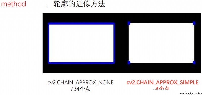
It can be seen that the latter saves a lot of computing space .
about cv2.drawContours( ):
r=cv2.drawContours(o, contours, contourIdx, color[, thickness])
r : Target image , Directly modify the pixels of the target , Implement drawing .
o : original image
contours : The edge array that needs to be drawn .
contourIdx : The edge index that needs to be drawn , If all are drawn, it is -1.
color : The color of the painting , by BGR Format Scalar .
thickness : Optional , Plotted density , That is, the thickness of the brush used to draw the outline .
import cv2import numpy as npo = cv2.imread('image\\boyun.png') gray = cv2.cvtColor(o,cv2.COLOR_BGR2GRAY) ret, binary = cv2.threshold(gray,127,255,cv2.THRESH_BINARY) image,contours, hierarchy =cv2.findContours(binary,cv2.RETR_TREE, cv2.CHAIN_APPROX_SIMPLE) co=o.copy()r=cv2.drawContours(co,contours,-1,(0,0,255),1) cv2.imshow("original",o)cv2.imshow("result",r)cv2.waitKey()cv2.destroyAllWindows()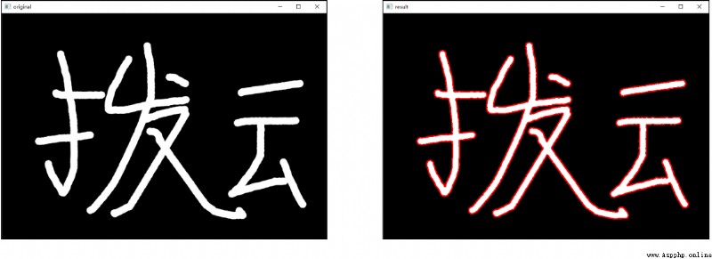
For multiple profiles , We can also specify which outline to draw .
gray = cv2.cvtColor(o,cv2.COLOR_BGR2GRAY) ret, binary = cv2.threshold(gray,127,255,cv2.THRESH_BINARY) image,contours, hierarchy = cv2.findContours(binary,cv2.RETR_TREE,cv2.CHAIN_APPROX_SIMPLE) co=o.copy()r=cv2.drawContours(co,contours,0,(0,0,255),6)
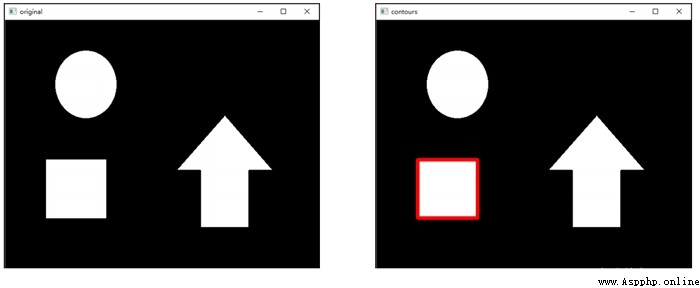
If I set it to -1, Then it is all displayed !!!
When there are burrs in the contour , We want to be able to do contour approximation , Remove burrs , The general idea is to replace the curve with a straight line , But there is a length threshold that needs to be set by yourself .
We can also do additional operations , For example, circumscribed rectangle , Circumcircle , Outer ellipse, etc .
img = cv2.imread('contours.png')gray = cv2.cvtColor(img, cv2.COLOR_BGR2GRAY)ret, thresh = cv2.threshold(gray, 127, 255, cv2.THRESH_BINARY)binary, contours, hierarchy = cv2.findContours(thresh, cv2.RETR_TREE, cv2.CHAIN_APPROX_NONE)cnt = contours[0]x,y,w,h = cv2.boundingRect(cnt)img = cv2.rectangle(img,(x,y),(x+w,y+h),(0,255,0),2)cv_show(img,'img')area = cv2.contourArea(cnt)x, y, w, h = cv2.boundingRect(cnt)rect_area = w * hextent = float(area) / rect_areaprint (' The ratio of contour area to boundary rectangle ',extent) Circumcircle (x,y),radius = cv2.minEnclosingCircle(cnt)center = (int(x),int(y))radius = int(radius)img = cv2.circle(img,center,radius,(0,255,0),2)cv_show(img,'img')Template matching is very similar to convolution , The template slides from the origin on the original image , Computing templates and ( Where the image is covered by the template ) The degree of difference , The calculation of the degree of difference is in opencv There are six in the , Then put the results of each calculation into a matrix , Output as a result . If the original figure is AXB size , And the template is axb size , Then the output matrix is (A-a+1)x(B-b+1).
TM_SQDIFF: The square is different , The smaller the calculated value , The more relevant
TM_CCORR: Calculate correlation , The larger the calculated value , The more relevant
TM_CCOEFF: Calculate the correlation coefficient , The larger the calculated value , The more relevant
TM_SQDIFF_NORMED: Calculating the normalized square is different , The closer the calculated value is to 0, The more relevant
TM_CCORR_NORMED: Calculate the normalized correlation , The closer the calculated value is to 1, The more relevant
TM_CCOEFF_NORMED: Calculate the normalized correlation coefficient , The closer the calculated value is to 1, The more relevant
That's about “python OpenCV Example analysis of image pyramid ” The content of this article , I believe we all have a certain understanding , I hope the content shared by Xiaobian will be helpful to you , If you want to know more about it , Please pay attention to the Yisu cloud industry information channel .