Preface
gradient
Forward propagation
Back propagation
Start training
PrefaceIn this article , Ready to use Python A fully connected neural network is implemented from scratch . You may ask , Why do you need to implement it yourself , There are many libraries and frameworks that can do this for us , such as Tensorflow、Pytorch etc. . I just want to say that I can only realize it myself , It's your own .
I think how much I have been engaged in the work related to neural networks since I came into contact with them today 2、3 Years. , Among them, try to use tensorflow or pytorch Framework to implement some classic networks . However, the mechanism behind the back propagation is still vague .
gradientGradient is the fastest rising direction of a function , The fastest direction means that the shape of the direction function is very steep , That is also the direction in which the function drops fastest .
Although there are some theories 、 Gradient vanishing and node saturation can output a 1、2、3 But there is still no confidence to study deeply , After all, I haven't realized a back propagation and complete training process by myself . So the feeling is still floating on the surface , Know why but .
Because I have a period of free time recently 、 So I will take advantage of this break to sort out this part of knowledge 、 Learn more about
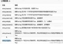
Type symbol description expression dimension Scalar n^LnL It means the first one L The number of neurons in this layer vector B^LBL It means the first one L Layer bias n^L \times 1nL×1 matrix W^LWL It means the first one L The weight of the layer n^L \times n^LnL×nL vector Z^LZL It means the first one L Layer input to the activation function Z^L=W^LA^{(L-1)} + B^LZL=WLA(L−1)+BLn^L \times 1nL×1 vector A^LAL It means the first one L Layer output value A^L = \sigma(Z^L)AL=σ(ZL)n^L \times 1nL×1We all probably know the process of training neural networks , Is to update network parameters , The direction of the update is to reduce the value of the loss function . That is to transform the learning problem into an optimization problem . So how to update parameters ? We need to calculate the derivative of the training parameters relative to the loss function , Then we solve the gradient , Then the gradient descent method is used to update the parameters , This iterative process , An optimal solution can be found to minimize the loss function .
We know that back propagation is mainly used to settle the derivatives of loss function relative to weight and bias
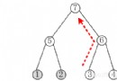
May have heard or read , A lot of information about the transmission of errors through back propagation in the network . And then according to the neurons w and b Contribution to deviation . That is, the error is distributed to each neuron . But the error here (error) What does that mean ? What is the exact definition of this error ? The answer is that these errors are contributed by each layer of neural network , And the error of a certain layer is shared on the basis of the error of subsequent layers , In the Internet  Layer error
  To express .
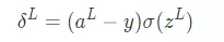
Back propagation is based on 4 Of a basic equation , The error is calculated from these equations  And the loss function , Here will be this 4 The equations are listed one by one
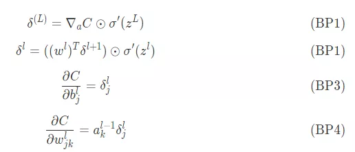
About how to interpret this 4 An equation , Later, I would like to use a share to explain .
class NeuralNetwork(object): def __init__(self): pass def forward(self,x): # Return to the forward propagation Z That is to say w and b A linear combination , Enter the value before activating the function # Returns the output value of the activation function A # z_s , a_s pass def backward(self,y,z_s,a_s): # Returns the derivative of the learning parameter in the forward propagation dw db pass def train(self,x,y,batch_size=10,epochs=100,lr=0.001): passWe are all neural network learning process , That's the training process . There are mainly two stages Forward propagation and Back propagation
In the forward propagation function , It mainly calculates the propagation Z and A, About Z and A See the table above for details
Calculating learnable variables in back propagation w and b The derivative of
def __init__(self,layers = [2 , 10, 1], activations=['sigmoid', 'sigmoid']): assert(len(layers) == len(activations)+1) self.layers = layers self.activations = activations self.weights = [] self.biases = [] for i in range(len(layers)-1): self.weights.append(np.random.randn(layers[i+1], layers[i])) self.biases.append(np.random.randn(layers[i+1], 1))layers Parameter is used to specify the number of neurons in each layer
activations Specify activation functions for each layer , That is to say 
To simply read the code assert(len(layers) == len(activations)+1)
for i in range(len(layers)-1): self.weights.append(np.random.randn(layers[i+1], layers[i])) self.biases.append(np.random.randn(layers[i+1], 1))Because the weights connect the neurons of each layer w and b , The equation between two layers , The above code is right
Forward propagation
def feedforward(self, x): # Returns the forward propagating value a = np.copy(x) z_s = [] a_s = [a] for i in range(len(self.weights)): activation_function = self.getActivationFunction(self.activations[i]) z_s.append(self.weights[i].dot(a) + self.biases[i]) a = activation_function(z_s[-1]) a_s.append(a) return (z_s, a_s) Here is the activation function , The return value of this function is a function , stay python use lambda To return a function , Here is a foreshadowing , It will be modified later .
@staticmethod def getActivationFunction(name): if(name == 'sigmoid'): return lambda x : np.exp(x)/(1+np.exp(x)) elif(name == 'linear'): return lambda x : x elif(name == 'relu'): def relu(x): y = np.copy(x) y[y<0] = 0 return y return relu else: print('Unknown activation function. linear is used') return lambda x: x[@staticmethod]def getDerivitiveActivationFunction(name): if(name == 'sigmoid'): sig = lambda x : np.exp(x)/(1+np.exp(x)) return lambda x :sig(x)*(1-sig(x)) elif(name == 'linear'): return lambda x: 1 elif(name == 'relu'): def relu_diff(x): y = np.copy(x) y[y>=0] = 1 y[y<0] = 0 return y return relu_diff else: print('Unknown activation function. linear is used') return lambda x: 1 Back propagation This is the focus of this sharing
def backpropagation(self,y, z_s, a_s): dw = [] # dC/dW db = [] # dC/dB deltas = [None] * len(self.weights) # delta = dC/dZ Calculate the error of each layer # The last layer of error deltas[-1] = ((y-a_s[-1])*(self.getDerivitiveActivationFunction(self.activations[-1]))(z_s[-1])) # Back propagation for i in reversed(range(len(deltas)-1)): deltas[i] = self.weights[i+1].T.dot(deltas[i+1])*(self.getDerivitiveActivationFunction(self.activations[i])(z_s[i])) #a= [print(d.shape) for d in deltas] batch_size = y.shape[1] db = [d.dot(np.ones((batch_size,1)))/float(batch_size) for d in deltas] dw = [d.dot(a_s[i].T)/float(batch_size) for i,d in enumerate(deltas)] # Return to weight (weight) matrix and Offset vector (biases) return dw, dbFirst, calculate the error of the last layer according to BP1 The equation gives us the following formula
deltas[-1] = ((y-a_s[-1])*(self.getDerivitiveActivationFunction(self.activations[-1]))(z_s[-1]))
Next, based on the  Error to calculate the current layer

batch_size = y.shape[1]db = [d.dot(np.ones((batch_size,1)))/float(batch_size) for d in deltas]dw = [d.dot(a_s[i].T)/float(batch_size) for i,d in enumerate(deltas)]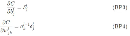
def train(self, x, y, batch_size=10, epochs=100, lr = 0.01):# update weights and biases based on the output for e in range(epochs): i=0 while(i<len(y)): x_batch = x[i:i+batch_size] y_batch = y[i:i+batch_size] i = i+batch_size z_s, a_s = self.feedforward(x_batch) dw, db = self.backpropagation(y_batch, z_s, a_s) self.weights = [w+lr*dweight for w,dweight in zip(self.weights, dw)] self.biases = [w+lr*dbias for w,dbias in zip(self.biases, db)] # print("loss = {}".format(np.linalg.norm(a_s[-1]-y_batch) ))This is about Python This is the end of the article on implementing a fully connected neural network , More about Python Please search the previous articles of SDN or continue to browse the related articles below. I hope you will support SDN more in the future !