一、單目三維重建概述
二、實現過程
(1)相機的標定
(2)圖像特征提取及匹配
(3)三維重建
三、結論
四、代碼
總結
一、單目三維重建概述客觀世界的物體是三維的,而我們用攝像機獲取的圖像是二維的,但是我們可以通過二維圖像感知目標的三維信息。三維重建技術是以一定的方式處理圖像進而得到計算機能夠識別的三維信息,由此對目標進行分析。而單目三維重建則是根據單個攝像頭的運動來模擬雙目視覺,從而獲得物體在空間中的三維視覺信息,其中,單目即指單個攝像頭。
二、實現過程在對物體進行單目三維重建的過程中,相關運行環境如下:
matplotlib 3.3.4
numpy 1.19.5
opencv-contrib-python 3.4.2.16
opencv-python 3.4.2.16
pillow 8.2.0
python 3.6.2
其重建主要包含以下步驟:
(1)相機的標定
(2)圖像特征提取及匹配
(3)三維重建
接下來,我們來詳細看下每個步驟的具體實現:
(1)相機的標定在我們日常生活中有很多相機,如手機上的相機、數碼相機及功能模塊型相機等等,每一個相機的參數都是不同的,即相機拍出的照片的分辨率、模式等。假設我們在進行物體三維重建的時候,事先並不知道我們相機的矩陣參數,那麼,我們就應當計算出相機的矩陣參數,這一個步驟就叫做相機的標定。相機標定的相關原理我就不介紹了,網上很多人都講解的挺詳細的。其標定的具體實現如下:
def camera_calibration(ImagePath): # 循環中斷 criteria = (cv2.TERM_CRITERIA_EPS + cv2.TERM_CRITERIA_MAX_ITER, 30, 0.001) # 棋盤格尺寸(棋盤格的交叉點的個數) row = 11 column = 8 objpoint = np.zeros((row * column, 3), np.float32) objpoint[:, :2] = np.mgrid[0:row, 0:column].T.reshape(-1, 2) objpoints = [] # 3d point in real world space imgpoints = [] # 2d points in image plane. batch_images = glob.glob(ImagePath + '/*.jpg') for i, fname in enumerate(batch_images): img = cv2.imread(batch_images[i]) imgGray = cv2.cvtColor(img, cv2.COLOR_BGR2GRAY) # find chess board corners ret, corners = cv2.findChessboardCorners(imgGray, (row, column), None) # if found, add object points, image points (after refining them) if ret: objpoints.append(objpoint) corners2 = cv2.cornerSubPix(imgGray, corners, (11, 11), (-1, -1), criteria) imgpoints.append(corners2) # Draw and display the corners img = cv2.drawChessboardCorners(img, (row, column), corners2, ret) cv2.imwrite('Checkerboard_Image/Temp_JPG/Temp_' + str(i) + '.jpg', img) print("成功提取:", len(batch_images), "張圖片角點!") ret, mtx, dist, rvecs, tvecs = cv2.calibrateCamera(objpoints, imgpoints, imgGray.shape[::-1], None, None)其中,cv2.calibrateCamera函數求出的mtx矩陣即為K矩陣。
當修改好相應參數並完成標定後,我們可以輸出棋盤格的角點圖片來看看是否已成功提取棋盤格的角點,輸出角點圖如下:
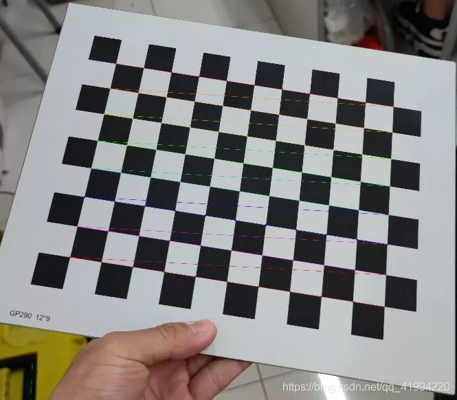
圖1:棋盤格角點提取
(2)圖像特征提取及匹配在整個三維重建的過程中,這一步是最為關鍵的,也是最為復雜的一步,圖片特征提取的好壞決定了你最後的重建效果。
在圖片特征點提取算法中,有三種算法較為常用,分別為:SIFT算法、SURF算法以及ORB算法。通過綜合分析對比,我們在這一步中采取SURF算法來對圖片的特征點進行提取。三種算法的特征點提取效果對比如果大家感興趣可以去網上搜來看下,在此就不逐一對比了。具體實現如下:
def epipolar_geometric(Images_Path, K): IMG = glob.glob(Images_Path) img1, img2 = cv2.imread(IMG[0]), cv2.imread(IMG[1]) img1_gray = cv2.cvtColor(img1, cv2.COLOR_BGR2GRAY) img2_gray = cv2.cvtColor(img2, cv2.COLOR_BGR2GRAY) # Initiate SURF detector SURF = cv2.xfeatures2d_SURF.create() # compute keypoint & descriptions keypoint1, descriptor1 = SURF.detectAndCompute(img1_gray, None) keypoint2, descriptor2 = SURF.detectAndCompute(img2_gray, None) print("角點數量:", len(keypoint1), len(keypoint2)) # Find point matches bf = cv2.BFMatcher(cv2.NORM_L2, crossCheck=True) matches = bf.match(descriptor1, descriptor2) print("匹配點數量:", len(matches)) src_pts = np.asarray([keypoint1[m.queryIdx].pt for m in matches]) dst_pts = np.asarray([keypoint2[m.trainIdx].pt for m in matches]) # plot knn_image = cv2.drawMatches(img1_gray, keypoint1, img2_gray, keypoint2, matches[:-1], None, flags=2) image_ = Image.fromarray(np.uint8(knn_image)) image_.save("MatchesImage.jpg") # Constrain matches to fit homography retval, mask = cv2.findHomography(src_pts, dst_pts, cv2.RANSAC, 100.0) # We select only inlier points points1 = src_pts[mask.ravel() == 1] points2 = dst_pts[mask.ravel() == 1]找到的特征點如下:
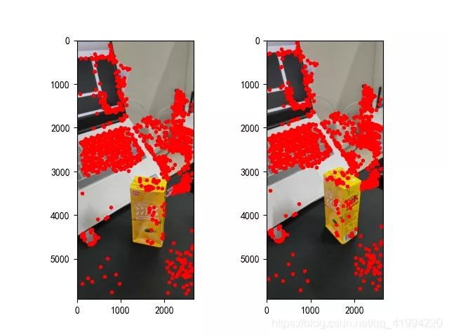
圖2:特征點提取
(3)三維重建我們找到圖片的特征點並相互匹配後,則可以開始進行三維重建了,具體實現如下:
points1 = cart2hom(points1.T)points2 = cart2hom(points2.T)# plotfig, ax = plt.subplots(1, 2)ax[0].autoscale_view('tight')ax[0].imshow(cv2.cvtColor(img1, cv2.COLOR_BGR2RGB))ax[0].plot(points1[0], points1[1], 'r.')ax[1].autoscale_view('tight')ax[1].imshow(cv2.cvtColor(img2, cv2.COLOR_BGR2RGB))ax[1].plot(points2[0], points2[1], 'r.')plt.savefig('MatchesPoints.jpg')fig.show()# points1n = np.dot(np.linalg.inv(K), points1)points2n = np.dot(np.linalg.inv(K), points2)E = compute_essential_normalized(points1n, points2n)print('Computed essential matrix:', (-E / E[0][1]))P1 = np.array([[1, 0, 0, 0], [0, 1, 0, 0], [0, 0, 1, 0]])P2s = compute_P_from_essential(E)ind = -1for i, P2 in enumerate(P2s): # Find the correct camera parameters d1 = reconstruct_one_point(points1n[:, 0], points2n[:, 0], P1, P2) # Convert P2 from camera view to world view P2_homogenous = np.linalg.inv(np.vstack([P2, [0, 0, 0, 1]])) d2 = np.dot(P2_homogenous[:3, :4], d1) if d1[2] > 0 and d2[2] > 0: ind = iP2 = np.linalg.inv(np.vstack([P2s[ind], [0, 0, 0, 1]]))[:3, :4]Points3D = linear_triangulation(points1n, points2n, P1, P2)fig = plt.figure()fig.suptitle('3D reconstructed', fontsize=16)ax = fig.gca(projection='3d')ax.plot(Points3D[0], Points3D[1], Points3D[2], 'b.')ax.set_xlabel('x axis')ax.set_ylabel('y axis')ax.set_zlabel('z axis')ax.view_init(elev=135, azim=90)plt.savefig('Reconstruction.jpg')plt.show()其重建效果如下(效果一般):
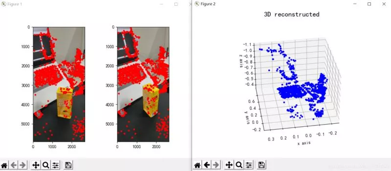
圖3:三維重建
三、結論從重建的結果來看,單目三維重建效果一般,我認為可能與這幾方面因素有關:
(1)圖片拍攝形式。如果是進行單目三維重建任務,在拍攝圖片時最好保持平行移動相機,且最好正面拍攝,即不要斜著拍或特異角度進行拍攝;
(2)拍攝時周邊環境干擾。選取拍攝的地點最好保持單一,減少無關物體的干擾;
(3)拍攝光源問題。選取的拍照場地要保證合適的亮度(具體情況要試才知道你們的光源是否達標),還有就是移動相機的時候也要保證前一時刻和此時刻的光源一致性。
其實,單目三維重建的效果確實一般,就算將各方面情況都拉滿,可能得到的重建效果也不是特別好。或者我們可以考慮采用雙目三維重建,雙目三維重建效果肯定是要比單目的效果好的,在實現是也就麻煩一(億)點點,哈哈。其實也沒有多太多的操作,主要就是整兩個相機拍攝和標定兩個相機麻煩點,其他的都還好。
四、代碼本次實驗的全部代碼如下:
GitHub:https://github.com/DeepVegChicken/Learning-3DReconstruction
import cv2import jsonimport numpy as npimport globfrom PIL import Imageimport matplotlib.pyplot as pltplt.rcParams['font.sans-serif'] = ['SimHei']plt.rcParams['axes.unicode_minus'] = Falsedef cart2hom(arr): """ Convert catesian to homogenous points by appending a row of 1s :param arr: array of shape (num_dimension x num_points) :returns: array of shape ((num_dimension+1) x num_points) """ if arr.ndim == 1: return np.hstack([arr, 1]) return np.asarray(np.vstack([arr, np.ones(arr.shape[1])]))def compute_P_from_essential(E): """ Compute the second camera matrix (assuming P1 = [I 0]) from an essential matrix. E = [t]R :returns: list of 4 possible camera matrices. """ U, S, V = np.linalg.svd(E) # Ensure rotation matrix are right-handed with positive determinant if np.linalg.det(np.dot(U, V)) < 0: V = -V # create 4 possible camera matrices (Hartley p 258) W = np.array([[0, -1, 0], [1, 0, 0], [0, 0, 1]]) P2s = [np.vstack((np.dot(U, np.dot(W, V)).T, U[:, 2])).T, np.vstack((np.dot(U, np.dot(W, V)).T, -U[:, 2])).T, np.vstack((np.dot(U, np.dot(W.T, V)).T, U[:, 2])).T, np.vstack((np.dot(U, np.dot(W.T, V)).T, -U[:, 2])).T] return P2sdef correspondence_matrix(p1, p2): p1x, p1y = p1[:2] p2x, p2y = p2[:2] return np.array([ p1x * p2x, p1x * p2y, p1x, p1y * p2x, p1y * p2y, p1y, p2x, p2y, np.ones(len(p1x)) ]).T return np.array([ p2x * p1x, p2x * p1y, p2x, p2y * p1x, p2y * p1y, p2y, p1x, p1y, np.ones(len(p1x)) ]).Tdef scale_and_translate_points(points): """ Scale and translate image points so that centroid of the points are at the origin and avg distance to the origin is equal to sqrt(2). :param points: array of homogenous point (3 x n) :returns: array of same input shape and its normalization matrix """ x = points[0] y = points[1] center = points.mean(axis=1) # mean of each row cx = x - center[0] # center the points cy = y - center[1] dist = np.sqrt(np.power(cx, 2) + np.power(cy, 2)) scale = np.sqrt(2) / dist.mean() norm3d = np.array([ [scale, 0, -scale * center[0]], [0, scale, -scale * center[1]], [0, 0, 1] ]) return np.dot(norm3d, points), norm3ddef compute_image_to_image_matrix(x1, x2, compute_essential=False): """ Compute the fundamental or essential matrix from corresponding points (x1, x2 3*n arrays) using the 8 point algorithm. Each row in the A matrix below is constructed as [x'*x, x'*y, x', y'*x, y'*y, y', x, y, 1] """ A = correspondence_matrix(x1, x2) # compute linear least square solution U, S, V = np.linalg.svd(A) F = V[-1].reshape(3, 3) # constrain F. Make rank 2 by zeroing out last singular value U, S, V = np.linalg.svd(F) S[-1] = 0 if compute_essential: S = [1, 1, 0] # Force rank 2 and equal eigenvalues F = np.dot(U, np.dot(np.diag(S), V)) return Fdef compute_normalized_image_to_image_matrix(p1, p2, compute_essential=False): """ Computes the fundamental or essential matrix from corresponding points using the normalized 8 point algorithm. :input p1, p2: corresponding points with shape 3 x n :returns: fundamental or essential matrix with shape 3 x 3 """ n = p1.shape[1] if p2.shape[1] != n: raise ValueError('Number of points do not match.') # preprocess image coordinates p1n, T1 = scale_and_translate_points(p1) p2n, T2 = scale_and_translate_points(p2) # compute F or E with the coordinates F = compute_image_to_image_matrix(p1n, p2n, compute_essential) # reverse preprocessing of coordinates # We know that P1' E P2 = 0 F = np.dot(T1.T, np.dot(F, T2)) return F / F[2, 2]def compute_fundamental_normalized(p1, p2): return compute_normalized_image_to_image_matrix(p1, p2)def compute_essential_normalized(p1, p2): return compute_normalized_image_to_image_matrix(p1, p2, compute_essential=True)def skew(x): """ Create a skew symmetric matrix *A* from a 3d vector *x*. Property: np.cross(A, v) == np.dot(x, v) :param x: 3d vector :returns: 3 x 3 skew symmetric matrix from *x* """ return np.array([ [0, -x[2], x[1]], [x[2], 0, -x[0]], [-x[1], x[0], 0] ])def reconstruct_one_point(pt1, pt2, m1, m2): """ pt1 and m1 * X are parallel and cross product = 0 pt1 x m1 * X = pt2 x m2 * X = 0 """ A = np.vstack([ np.dot(skew(pt1), m1), np.dot(skew(pt2), m2) ]) U, S, V = np.linalg.svd(A) P = np.ravel(V[-1, :4]) return P / P[3]def linear_triangulation(p1, p2, m1, m2): """ Linear triangulation (Hartley ch 12.2 pg 312) to find the 3D point X where p1 = m1 * X and p2 = m2 * X. Solve AX = 0. :param p1, p2: 2D points in homo. or catesian coordinates. Shape (3 x n) :param m1, m2: Camera matrices associated with p1 and p2. Shape (3 x 4) :returns: 4 x n homogenous 3d triangulated points """ num_points = p1.shape[1] res = np.ones((4, num_points)) for i in range(num_points): A = np.asarray([ (p1[0, i] * m1[2, :] - m1[0, :]), (p1[1, i] * m1[2, :] - m1[1, :]), (p2[0, i] * m2[2, :] - m2[0, :]), (p2[1, i] * m2[2, :] - m2[1, :]) ]) _, _, V = np.linalg.svd(A) X = V[-1, :4] res[:, i] = X / X[3] return resdef writetofile(dict, path): for index, item in enumerate(dict): dict[item] = np.array(dict[item]) dict[item] = dict[item].tolist() js = json.dumps(dict) with open(path, 'w') as f: f.write(js) print("參數已成功保存到文件")def readfromfile(path): with open(path, 'r') as f: js = f.read() mydict = json.loads(js) print("參數讀取成功") return mydictdef camera_calibration(SaveParamPath, ImagePath): # 循環中斷 criteria = (cv2.TERM_CRITERIA_EPS + cv2.TERM_CRITERIA_MAX_ITER, 30, 0.001) # 棋盤格尺寸 row = 11 column = 8 objpoint = np.zeros((row * column, 3), np.float32) objpoint[:, :2] = np.mgrid[0:row, 0:column].T.reshape(-1, 2) objpoints = [] # 3d point in real world space imgpoints = [] # 2d points in image plane. batch_images = glob.glob(ImagePath + '/*.jpg') for i, fname in enumerate(batch_images): img = cv2.imread(batch_images[i]) imgGray = cv2.cvtColor(img, cv2.COLOR_BGR2GRAY) # find chess board corners ret, corners = cv2.findChessboardCorners(imgGray, (row, column), None) # if found, add object points, image points (after refining them) if ret: objpoints.append(objpoint) corners2 = cv2.cornerSubPix(imgGray, corners, (11, 11), (-1, -1), criteria) imgpoints.append(corners2) # Draw and display the corners img = cv2.drawChessboardCorners(img, (row, column), corners2, ret) cv2.imwrite('Checkerboard_Image/Temp_JPG/Temp_' + str(i) + '.jpg', img) print("成功提取:", len(batch_images), "張圖片角點!") ret, mtx, dist, rvecs, tvecs = cv2.calibrateCamera(objpoints, imgpoints, imgGray.shape[::-1], None, None) dict = {'ret': ret, 'mtx': mtx, 'dist': dist, 'rvecs': rvecs, 'tvecs': tvecs} writetofile(dict, SaveParamPath) meanError = 0 for i in range(len(objpoints)): imgpoints2, _ = cv2.projectPoints(objpoints[i], rvecs[i], tvecs[i], mtx, dist) error = cv2.norm(imgpoints[i], imgpoints2, cv2.NORM_L2) / len(imgpoints2) meanError += error print("total error: ", meanError / len(objpoints))def epipolar_geometric(Images_Path, K): IMG = glob.glob(Images_Path) img1, img2 = cv2.imread(IMG[0]), cv2.imread(IMG[1]) img1_gray = cv2.cvtColor(img1, cv2.COLOR_BGR2GRAY) img2_gray = cv2.cvtColor(img2, cv2.COLOR_BGR2GRAY) # Initiate SURF detector SURF = cv2.xfeatures2d_SURF.create() # compute keypoint & descriptions keypoint1, descriptor1 = SURF.detectAndCompute(img1_gray, None) keypoint2, descriptor2 = SURF.detectAndCompute(img2_gray, None) print("角點數量:", len(keypoint1), len(keypoint2)) # Find point matches bf = cv2.BFMatcher(cv2.NORM_L2, crossCheck=True) matches = bf.match(descriptor1, descriptor2) print("匹配點數量:", len(matches)) src_pts = np.asarray([keypoint1[m.queryIdx].pt for m in matches]) dst_pts = np.asarray([keypoint2[m.trainIdx].pt for m in matches]) # plot knn_image = cv2.drawMatches(img1_gray, keypoint1, img2_gray, keypoint2, matches[:-1], None, flags=2) image_ = Image.fromarray(np.uint8(knn_image)) image_.save("MatchesImage.jpg") # Constrain matches to fit homography retval, mask = cv2.findHomography(src_pts, dst_pts, cv2.RANSAC, 100.0) # We select only inlier points points1 = src_pts[mask.ravel() == 1] points2 = dst_pts[mask.ravel() == 1] points1 = cart2hom(points1.T) points2 = cart2hom(points2.T) # plot fig, ax = plt.subplots(1, 2) ax[0].autoscale_view('tight') ax[0].imshow(cv2.cvtColor(img1, cv2.COLOR_BGR2RGB)) ax[0].plot(points1[0], points1[1], 'r.') ax[1].autoscale_view('tight') ax[1].imshow(cv2.cvtColor(img2, cv2.COLOR_BGR2RGB)) ax[1].plot(points2[0], points2[1], 'r.') plt.savefig('MatchesPoints.jpg') fig.show() # points1n = np.dot(np.linalg.inv(K), points1) points2n = np.dot(np.linalg.inv(K), points2) E = compute_essential_normalized(points1n, points2n) print('Computed essential matrix:', (-E / E[0][1])) P1 = np.array([[1, 0, 0, 0], [0, 1, 0, 0], [0, 0, 1, 0]]) P2s = compute_P_from_essential(E) ind = -1 for i, P2 in enumerate(P2s): # Find the correct camera parameters d1 = reconstruct_one_point(points1n[:, 0], points2n[:, 0], P1, P2) # Convert P2 from camera view to world view P2_homogenous = np.linalg.inv(np.vstack([P2, [0, 0, 0, 1]])) d2 = np.dot(P2_homogenous[:3, :4], d1) if d1[2] > 0 and d2[2] > 0: ind = i P2 = np.linalg.inv(np.vstack([P2s[ind], [0, 0, 0, 1]]))[:3, :4] Points3D = linear_triangulation(points1n, points2n, P1, P2) return Points3Ddef main(): CameraParam_Path = 'CameraParam.txt' CheckerboardImage_Path = 'Checkerboard_Image' Images_Path = 'SubstitutionCalibration_Image/*.jpg' # 計算相機參數 camera_calibration(CameraParam_Path, CheckerboardImage_Path) # 讀取相機參數 config = readfromfile(CameraParam_Path) K = np.array(config['mtx']) # 計算3D點 Points3D = epipolar_geometric(Images_Path, K) # 重建3D點 fig = plt.figure() fig.suptitle('3D reconstructed', fontsize=16) ax = fig.gca(projection='3d') ax.plot(Points3D[0], Points3D[1], Points3D[2], 'b.') ax.set_xlabel('x axis') ax.set_ylabel('y axis') ax.set_zlabel('z axis') ax.view_init(elev=135, azim=90) plt.savefig('Reconstruction.jpg') plt.show()if __name__ == '__main__': main()總結到此這篇關於如何基於python實現單目三維重建的文章就介紹到這了,更多相關python單目三維重建內容請搜索軟件開發網以前的文章或繼續浏覽下面的相關文章希望大家以後多多支持軟件開發網!