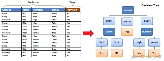
人工智能

第五章 車輛評級分類與cart分類樹

一、決策樹分類

1. 算法核心原理

• 決策樹的核心思想：相似的輸入產生相似的輸出。

2. 決策樹的關鍵問題

• 這麼多特征，使用哪個特征先進行子表劃分？

3. CART 分類樹

• CART 分類樹算法對每個特征進行二分，尋找分割點時使用基尼系數來表達數據集的不純度，基尼系數越小，不純度越低，數據集劃分的效果越好。
• CART 分類樹劃分子表的過程：
  • 針對每個特征，基於基尼系數計算最優分割值。在計算出來的各個特征的每個分割值對數據集 D D D的基尼系數中，選擇基尼系數最小的特征A和對應的分割值a。根據這個最優特征和最優分割值，把數據集劃分成兩部分 D 1 D_1 D1​和 D 2 D_2 D2​，同時建立當前節點的左右節點，左節點的數據集 D D D為 D 1 D_1 D1​，右節點的數據集 D D D為 D 2 D_2 D2​.對左右節點的子節點遞歸調用這個過程，生成決策樹。
• 而 CART 分類樹也基於基尼系數來決定子表劃分所選特征的次序。

4. 基尼系數

• 對於樣本D，個數為|D|，假設K個類別，第k個類別的數量為 C k C_k Ck​，則樣本D的基尼系數表達式：
  G i n i ( D ) = 1 − ∑ i = 1 K ( ∣ C k ∣ ∣ D ∣ ) 2 Gini(D) = 1 - \sum_{i=1}^K \left(\frac{|C_k|}{|D|}\right)^2 Gini(D)=1−i=1∑K​(∣D∣∣Ck​∣​)2
• 有100個樣本( D 1 D_1 D1​)包含A與B兩個類別，數量分別為40與60，Gini( D 1 D_1 D1​) = ?
  1 − ( ( ∣ 40 ∣ ∣ 100 ∣ ) 2 + ( ∣ 60 ∣ ∣ 100 ∣ ) 2 ) = 1 − ( 0.16 + 0.36 ) = 0.48 1 - \left( \left(\frac{|40|}{|100|}\right)^2 + \left( \frac{|60|}{|100|}\right)^2 \right) = 1 - (0.16 + 0.36) = 0.48 1−((∣100∣∣40∣​)2+(∣100∣∣60∣​)2)=1−(0.16+0.36)=0.48
• 有100個樣本( D 2 D_2 D2​)包含A與B兩個類別，數量分別為10與90，Gini( D 2 D_2 D2​) = ?
  1 − ( ( ∣ 10 ∣ ∣ 100 ∣ ) 2 + ( ∣ 90 ∣ ∣ 100 ∣ ) 2 ) = 1 − ( 0.01 + 0.81 ) = 0.18 1 - \left( \left( \frac{|10|}{|100|}\right)^2 + \left( \frac{|90|}{|100|}\right)^2 \right) = 1 - (0.01 + 0.81) = 0.18 1−((∣100∣∣10∣​)2+(∣100∣∣90∣​)2)=1−(0.01+0.81)=0.18
• 對於樣本D，個數為|D|，根據特征A的某個值a，把D分成 D 1 D_1 D1​和 D 2 D_2 D2​，則在特征A的條件下，樣本D的基尼系數表達式為：
  G i n i ( D , A ) = ∣ D 1 ∣ ∣ D ∣ G i n i ( D 1 ) + ∣ D 2 ∣ ∣ D ∣ G i n i ( D 2 ) Gini(D,A) = \frac{|D_1|}{|D|} Gini(D_1) + \frac{|D_2|}{|D|} Gini(D_2) Gini(D,A)=∣D∣∣D1​∣​Gini(D1​)+∣D∣∣D2​∣​Gini(D2​)

5. 決策樹的生成過程

• 算法輸入訓練集D，基尼系數的阈值，樣本個數阈值。輸出決策樹T。
  • 對於當前節點的數據集為D，如果樣本個數小於阈值，則返回決策子樹，當前節點停止遞歸。
  • 計算樣本集D的基尼系數，如果基尼系數小於阈值，則返回決策樹子樹，當前節點停止遞歸。
  • 計算當前節點現有的各個特征的各個特征值對數據集D的基尼系數。
  • 在計算出來的各個特征的各個特征值對數據集D的基尼系數中，選擇基尼系數最小的特征A和對應的特征值a。根據這個最優特征和最優特征值，把數據集劃分成兩部分 D 1 D_1 D1​和 D 2 D_2 D2​，同時建立當前節點的左右節點，左節點的數據集D為 D 1 D_1 D1​，右節點的數據集D為 D 2 D_2 D2​。
  • 對左右的子節點遞歸的調用1-4步，生成決策樹。
• 預測過程：對生成的決策樹做預測的時候，假如測試集裡的樣本A落到了某個葉子節點，而節點裡有多個訓練樣本。則對於A的類別預測采用的是這個葉子節點裡概率最大的類別。

6. 決策樹分類實現

• 決策樹分類器模型相關 API：

import sklearn.tree as st
# 決策樹分類器
model = st.DecisionTreeClassifier(
max_depth=6, min_samples_split=3, random_state=7)
model.fit(train_x, train_y)

7. 鸢尾花案例

import sklearn.tree as st
model = st.DecisionTreeClassifier(max_depth=4, min_samples_split=3)
model.fit(train_x, train_y)
# 評估 模型准確率
pred_test_y = model.predict(test_x)
print((pred_test_y==test_y).sum() / test_y.size)
print(test_y.values)
""" 0.8666666666666667 [2 0 0 1 0 2 2 2 1 1 2 1 1 0 0] """

8. 集合模型分類實現

• 集合模型提供的常用分類器

import sklearn.ensemble as se
model = se.RandomForestClassifier(...) # 隨機森林分類器
model = se.AdaBoostClassifier(...) # AdaBoost分類器
model = se.GridientBoostingClassifier(...) # GBDT分類器

二、預測小汽車等級

• car.txt 樣本文件中統計了小汽車的常見特征信息及小汽車的分類，使用這些數據基於決策樹分類算法訓練模型預測小汽車等級。
• 汽車價格 維修費用 車門數量 載客數 後備箱 安全性 汽車級別
• 分析實現思路：
  • 加載數據。
  • 特征分析與特征工程。
  • 數據預處理（標簽編碼）。
  • 訓練模型。
  • 模型測試。

import numpy as np
import pandas as pd
data = pd.read_csv('car.txt', header=None) # 不想把第一行當做表頭
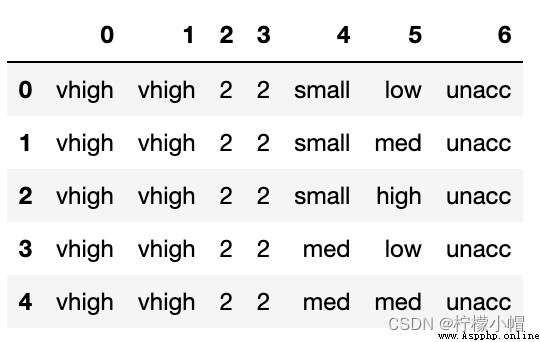
data.head()

data[0].value_counts() # 汽車價格分成4類，按類別劃分每個類別有432個樣本
""" vhigh 432 low 432 med 432 high 432 Name: 0, dtype: int64 """

• 確定：是分類問題，還是回歸問題？答：分類
• 選哪一個分類模型：邏輯回歸、決策樹、RF、GBDT、AdaBoost？答：RF（當然也可以嘗試其他模型）

# 針對當前這組數據完成標簽編碼預處理
import sklearn.preprocessing as sp
# 遍歷每一列數據
train_data = pd.DataFrame([])
encoders = {
}
for col_ind, col_val in data.items():
encoder = sp.LabelEncoder()
train_data[col_ind] = encoder.fit_transform(col_val)
encoders[col_ind] = encoder
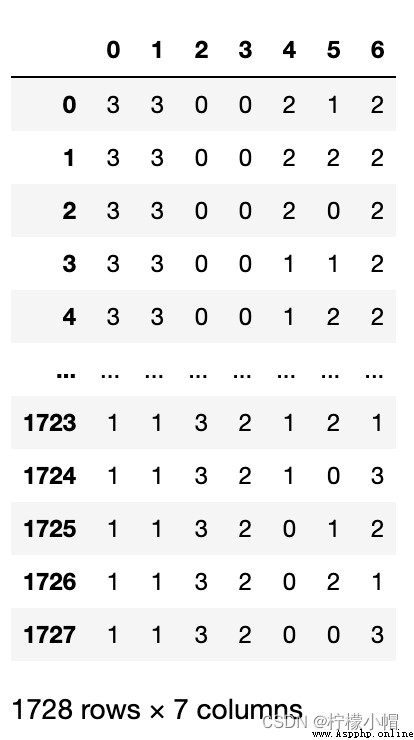
train_data

# 整理輸入集與輸出集
x, y = train_data.iloc[:, :-1], train_data[6]
x.shape, y.shape
""" ((1728, 6), (1728,)) """
# 創建分類模型
model = se.RandomForestClassifier(max_depth=6, n_estimators=400, random_state=7)
# 做5次交叉驗證，驗證一下這個模型是否可用
scores = ms.cross_val_score(model, x, y, cv=5, scoring='f1_weighted')
# 如果分數還可以，再正兒八經的訓練模型
print(scores.mean())
""" 0.7537201013972693 """
# 模型評估（先用訓練樣本進行模型評估）
model.fit(x, y)
pred_y = model.predict(x)
print(sm.classification_report(y, pred_y))
print(sm.confusion_matrix(y,pred_y)) # 把1類別的全歸到0類別裡了
""" precision recall f1-score support 0 0.77 0.82 0.79 384 1 0.00 0.00 0.00 69 2 0.95 0.99 0.97 1210 3 1.00 0.77 0.87 65 accuracy 0.91 1728 macro avg 0.68 0.65 0.66 1728 weighted avg 0.87 0.91 0.89 1728 [[ 315 0 69 0] [ 69 0 0 0] [ 11 0 1199 0] [ 15 0 0 50]] """
data = [
['high', 'med', '5more', '4', 'big', 'low', 'unacc'],
['high', 'high', '4', '4', 'med', 'med', 'acc'],
['low', 'low', '2', '4', 'small', 'high', 'good'],
['low', 'med', '3', '4', 'med', 'high', 'vgood']
]
test_data = pd.DataFrame(data)
for col_ind, col_val in test_data.items():
encoder = encoders[col_ind]
encoded_col = encoder.transform(col_val)
test_data[col_ind] = encoded_col
# 整理輸入集與輸出集
test_x, test_y = test_data.iloc[:,:-1], test_data[6]
pred_test_y = model.predict(test_x)
pred_test_y
""" array([2, 0, 0, 0]) """
encoders[6].inverse_transform(pred_test_y)
""" array(['unacc', 'acc', 'acc', 'acc'], dtype=object) """

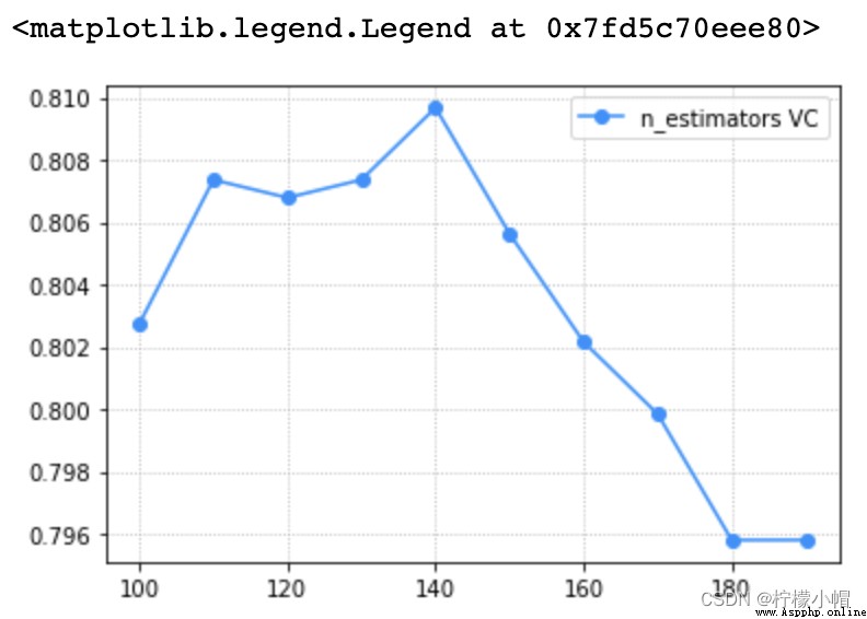
三、驗證曲線與學習曲線

1. 驗證曲線

• 驗證曲線描述的關系即是模型性能關於模型超參數的函數關系：
  • 模型性能 = f（超參數）

2. 驗證曲線實現

• sklearn 提供的驗證曲線 API：

train_scores, test_scores = ms.validation_curve(
model, # 模型
輸入集, 輸出集,
'n_estimators', # 超參數名
np.arange(50, 550, 50), # 超參數序列
cv=5 # 折疊數
)

• 返回train_scores與test_scores為每個超參數取值下的每次交叉驗證結果組成的得分矩陣。

3. 案例：預測小汽車等級調整參數

import numpy as np
import pandas as pd
data = pd.read_csv('car.txt', header=None) # 不想把第一行當做表頭
# 針對當前這組數據完成標簽編碼預處理
import sklearn.preprocessing as sp
import sklearn.ensemble as se
import sklearn.model_selection as ms
import sklearn.metrics as sm
# 遍歷每一列數據
train_data = pd.DataFrame([])
encoders = {
}
for col_ind, col_val in data.items():
encoder = sp.LabelEncoder()
train_data[col_ind] = encoder.fit_transform(col_val)
encoders[col_ind] = encoder
# 整理輸入集與輸出集
x, y = train_data.iloc[:, :-1], train_data[6]
# 創建分類模型（調參之後設定的參數值）
model = se.RandomForestClassifier(max_depth=9, n_estimators=140, random_state=7)
# 驗證曲線，選取最優超參數
import matplotlib.pyplot as plt
# params = np.arange(50, 550, 50)
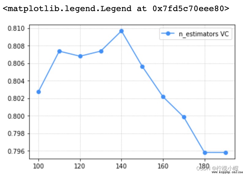
params = np.arange(100, 200, 10)
train_scores, test_scores = ms.validation_curve(model, x, y, param_name='n_estimators', param_range=params, cv=5)
scores = test_scores.mean(axis=1)
# 驗證曲線可視化
plt.grid(linestyle=':')
plt.plot(params, scores, 'o-', color='dodgerblue', label='n_estimators VC')
plt.legend()

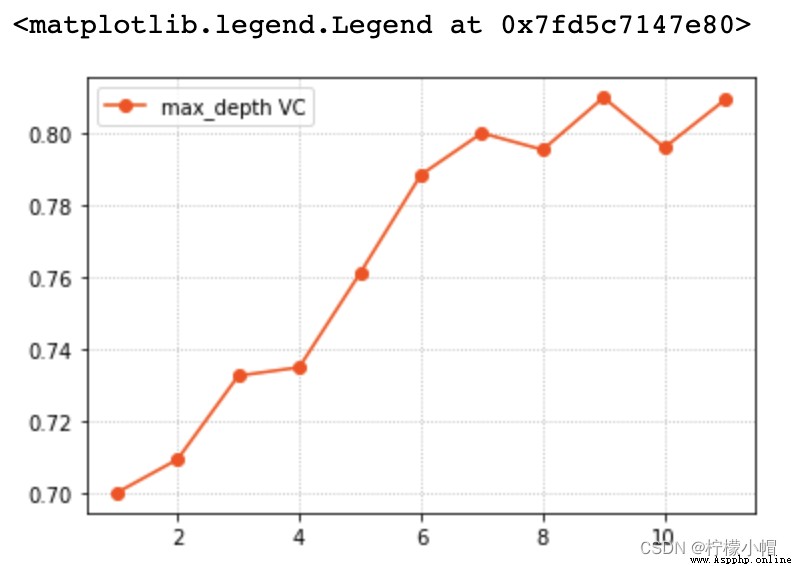
# 調整max_depth
params = np.arange(1, 12)
train_scores, test_scores = ms.validation_curve(model, x, y, param_name='max_depth', param_range=params, cv=5)
scores = test_scores.mean(axis=1)
# 驗證曲線可視化
plt.grid(linestyle=':')
plt.plot(params, scores, 'o-', color='orangered', label='max_depth VC')
plt.legend()

model.fit(x, y)
pred_y = model.predict(x)
print(sm.classification_report(y, pred_y))
print(sm.confusion_matrix(y,pred_y))
""" precision recall f1-score support 0 0.96 1.00 0.98 384 1 1.00 0.75 0.86 69 2 1.00 1.00 1.00 1210 3 0.94 1.00 0.97 65 accuracy 0.99 1728 macro avg 0.97 0.94 0.95 1728 weighted avg 0.99 0.99 0.99 1728 [[ 383 0 0 1] [ 14 52 0 3] [ 3 0 1207 0] [ 0 0 0 65]] """
data = [
['high', 'med', '5more', '4', 'big', 'low', 'unacc'],
['high', 'high', '4', '4', 'med', 'med', 'acc'],
['low', 'low', '2', '4', 'small', 'high', 'good'],
['low', 'med', '3', '4', 'med', 'high', 'vgood']
]
test_data = pd.DataFrame(data)
for col_ind, col_val in test_data.items():
encoder = encoders[col_ind]
encoded_col = encoder.transform(col_val)
test_data[col_ind] = encoded_col
# 整理輸入集與輸出集
test_x, test_y = test_data.iloc[:,:-1], test_data[6]
pred_test_y = model.predict(test_x)
encoders[6].inverse_transform(pred_test_y)
""" array(['unacc', 'acc', 'good', 'vgood'], dtype=object) """

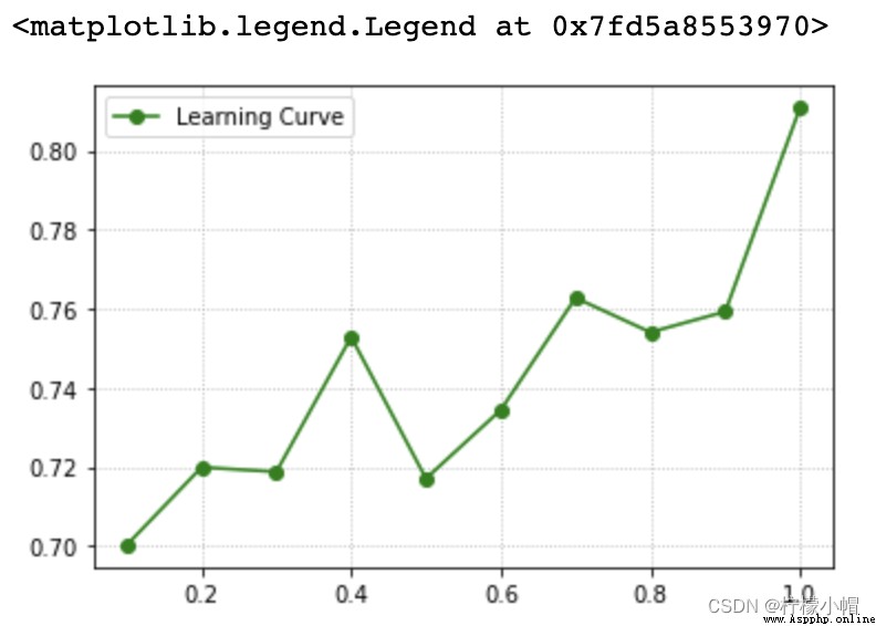
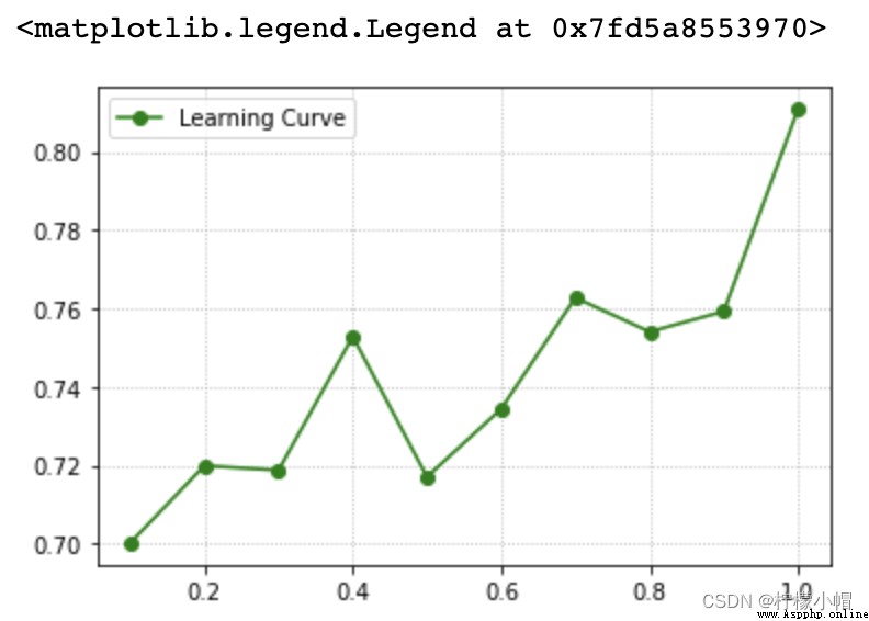
4. 學習曲線

• 學習曲線描述的關系即是模型性能關於訓練樣本量大小的函數關系：
  • 模型性能 = f（訓練集大小）

5. 學習曲線實現

• sklearn 提供的學習曲線 API：

train_scores, test_scores = ms.learning_curve(
model, # 模型
輸入集, 輸出集,
train_sizes=[0.9, 0.8, 0.7], # 訓練集大小序列
cv=5 # 折疊數
)

• 返回train_scores與test_scores為每個超參數取值下的每次交叉驗證結果組成的得分矩陣。

6. 案例：預測小汽車等級調整參數

params = np.arange(0.1, 1.1, 0.1)
_, train_scores, test_scores = ms.learning_curve(model, x, y, train_sizes=params, cv=5)
scores = test_scores.mean(axis = 1)
# 學習曲線可視化
plt.grid(linestyle=':')
plt.plot(params, scores, 'o-', color='green', label='Learning Curve')
plt.legend()

四、完整案例

import numpy as np
import pandas as pd
data = pd.read_csv('car.txt', header=None) # 不想把第一行當做表頭
data.head()
""" 0 1 2 3 4 5 6 0 vhigh vhigh 2 2 small low unacc 1 vhigh vhigh 2 2 small med unacc 2 vhigh vhigh 2 2 small high unacc 3 vhigh vhigh 2 2 med low unacc 4 vhigh vhigh 2 2 med med unacc """
# 確定：是分類問題，還是回歸問題？ 分類
# 選哪一個分類模型：邏輯回歸、決策樹、RF、GBDT、AdaBoost？ RF
# 針對當前這組數據完成標簽編碼預處理
import sklearn.preprocessing as sp
import sklearn.ensemble as se
import sklearn.model_selection as ms
import sklearn.metrics as sm
# 遍歷每一列數據
train_data = pd.DataFrame([])
encoders = {
}
for col_ind, col_val in data.items():
encoder = sp.LabelEncoder()
train_data[col_ind] = encoder.fit_transform(col_val)
encoders[col_ind] = encoder
# 整理輸入集與輸出集
x, y = train_data.iloc[:, :-1], train_data[6]
# 創建分類模型
model = se.RandomForestClassifier(max_depth=9, n_estimators=140, random_state=7)
# 驗證曲線，選取最優超參數
import matplotlib.pyplot as plt
# params = np.arange(50, 550, 50)
params = np.arange(100, 200, 10)
train_scores, test_scores = ms.validation_curve(model, x, y, param_name='n_estimators', param_range=params, cv=5)
scores = test_scores.mean(axis=1)
# 驗證曲線可視化
plt.grid(linestyle=':')
plt.plot(params, scores, 'o-', color='dodgerblue', label='n_estimators VC')
plt.legend()

# 調整max_depth
params = np.arange(1, 12)
train_scores, test_scores = ms.validation_curve(model, x, y, param_name='max_depth', param_range=params, cv=5)
scores = test_scores.mean(axis=1)
# 驗證曲線可視化
plt.grid(linestyle=':')
plt.plot(params, scores, 'o-', color='orangered', label='max_depth VC')
plt.legend()

# 學習曲線，選取最優訓練集大小
params = np.arange(0.1, 1.1, 0.1)
_, train_scores, test_scores = ms.learning_curve(model, x, y, train_sizes=params, cv=5)
scores = test_scores.mean(axis = 1)
# 學習曲線可視化
plt.grid(linestyle=':')
plt.plot(params, scores, 'o-', color='green', label='Learning Curve')
plt.legend()

# 模型評估（先用訓練樣本進行模型評估）
model.fit(x, y)
pred_y = model.predict(x)
print(sm.classification_report(y, pred_y))
print(sm.confusion_matrix(y,pred_y)) # 把1類別的全歸到0類別裡了
""" precision recall f1-score support 0 0.96 1.00 0.98 384 1 1.00 0.75 0.86 69 2 1.00 1.00 1.00 1210 3 0.94 1.00 0.97 65 accuracy 0.99 1728 macro avg 0.97 0.94 0.95 1728 weighted avg 0.99 0.99 0.99 1728 [[ 383 0 0 1] [ 14 52 0 3] [ 3 0 1207 0] [ 0 0 0 65]] """
data = [
['high', 'med', '5more', '4', 'big', 'low', 'unacc'],
['high', 'high', '4', '4', 'med', 'med', 'acc'],
['low', 'low', '2', '4', 'small', 'high', 'good'],
['low', 'med', '3', '4', 'med', 'high', 'vgood']
]
test_data = pd.DataFrame(data)
for col_ind, col_val in test_data.items():
encoder = encoders[col_ind]
encoded_col = encoder.transform(col_val)
test_data[col_ind] = encoded_col
# 整理輸入集與輸出集
test_x, test_y = test_data.iloc[:,:-1], test_data[6]
pred_test_y = model.predict(test_x)
encoders[6].inverse_transform(pred_test_y)
""" array(['unacc', 'acc', 'good', 'vgood'], dtype=object) """