Credit risk control is one of the most successful applications of data mining algorithms , This is because the data volume of the financial and credit industry is sufficient , The demand scenarios are clear and rich .
Credit risk control is simply to judge whether a person has borrowed money ( The repayment date of the following months ) Will you pay back the money on time . More professionally , Credit risk control is a comprehensive consideration of repayment ability and willingness , Lending on the basis of trust based on this prior judgment , This greatly improves the efficiency of financial business .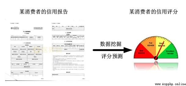
It is different from other industrial scenarios of machine learning , Finance is an extremely risk averse field , Its particularity lies in its emphasis on the interpretability and stability of the model . The common practice in the industry is to establish a set of rules and risk control models that can be explained and have stable effects based on mining multi-dimensional features / user / Act to make judgments and decisions .
among , about ( Before loan ) Risk control model before application , Also called application scorecard --A card .A Card is the key model of risk control , The industry consensus is that the application score card can cover 80% The credit risk of . In addition, there is the credit behavior scorecard B card 、 Collection Scorecard C card , And the anti fraud model .
A card (Application score card). The purpose is to predict when ( Apply for a credit card 、 Apply for a loan ) Quantitative evaluation of the applicant .B card (Behavior score card). The purpose is to predict the time point of use ( Get a loan 、 The duration of the credit card ) Probability of overdue within a certain time in the future .C card (Collection score card). The purpose is to predict the probability of repayment within a certain period of time after overdue and entering the collection stage .
A good feature , It is crucial for both models and rules . Like applying for a scorecard --A card , It can be mainly classified into the following 3 Aspect characteristics :
1、 Credit history : Number and amount of credit transactions 、 Income debt ratio 、 The number of credit inquiries 、 Credit history length 、 Number of new credit accounts opened 、 Quota utilization rate 、 Overdue times and amount 、 Type of credit product 、 Information on recovery .( The characteristics of credit transactions are often the most important , Without this part of information about historical repayment ability and willingness , Risk control models are usually discarded directly .)
2、 Basic data and transaction records : Age 、 Marital status 、 Education 、 Type of work and annual salary 、 Wage income 、 deposit AUM、 Assets situation 、 Provident fund and tax payment 、 Records of non credit transactions ( This category is mainly considered from the perspective of repayment ability . You can also verify the authenticity of the data and share the mobile phone number 、 ID number and other gang fraud information , Used to identify fraud risks . Need to pay attention to , Like gender 、 Skin colour 、 regional 、 race 、 Religious belief and other types of features should be used with caution , Maybe the model will work , But it will also lead to algorithm discrimination .)
3、 Public negative records : Such as bankruptcy liabilities 、 Civil judgment 、 administrative sanction 、 The court enforces 、 Blacklists involving gambling and fraud ( Such features do not necessarily yield data , And the degree of deletion is usually high , Contribution to the model is average , More from the willingness to repay / Consideration of fraud dimension )
In the practical part, we take the classic application Scorecard as an example , The data set of the personal loan default prediction competition of Zhongyuan bank , Use credit scoring python library --toad、 Tree model Lightgbm And logistic regression LR Make an application scoring model .( notes : Some financial terms involved in this article , Because of the space, I will not explain , Questions You can learn about it by Google .)
The definition of the application scoring model is mainly to determine the modeling samples and labels through a series of data analysis .
First , Add a few descriptions of financial risk control terms . If the concept is vague , You can go back and understand :
Number of overdue periods (M) : It refers to the overdue days between the actual repayment date and the repayment date , And the overdue status divided by interval .M Taken from the Month on Book The first word of .( notes : The interval division defined by different organizations may be different ) M0: Currently not overdue ( Or use C Express , Taken from the Current) M1: Within the time limit 1-30 Japan M2: Within the time limit 31-60 Japan M3: Within the time limit 61-90 Japan M4: Within the time limit 91-120 Japan M5: Within the time limit 121-150 Japan M6: Within the time limit 151-180 Japan M7+: Within the time limit 180 More than days
Observation points : Sample level time window . The point in time used to build the sample set ( Such as 2010 year 10 Users who apply for loans in January ), Different links have different definitions , More abstract , Here is an example : In case of application model , The observation point is defined as the user's loan application time , take 19 year 1-12 All the loan application orders in the month are used as the construction sample set ; If it's a loan behavior model , An observation point is defined as a specific date , If you take 19 year 6 month 15 The day is on loan 、 There is no overdue loan application order to build the sample set .
Observation period : Time window at feature level . Construct the relative time window of the feature , For example, before a user applies for a loan 12 months (2009 year 10 The month ends at 2010 year 10 The data before applying for the loan every month can be used , Average consumption amount of users 、 frequency 、 Loan times and other data characteristics ). The observation period is set for the feature alignment of each sample , The length is usually determined by the data . One thing to note is , Only this time Before applying Characteristic data of , Otherwise, data will be leaked ( Time goes by , Use the future to predict past phenomena ).
Performance period : Time window at label level . Define good and bad labels Y Time window of , Credit risk has natural lag , Because one month after the user borrowed money ( The first phase ) Just started paying back , It's possible that it took several instalments to pay off .
For ready-made game data , Time span of data characteristics ( Observation period )、 Data samples 、 Label definitions have been analyzed and determined in advance . But for real business , In fact, data samples and model definitions are also the key to applying for scorecards . After all, there may be no ready-made data and labels thrown to you in the actual scene ( The definition of good and bad , The business of some companies will be analyzed in advance for the modeler ), Then just run a classification model .
Determine the sample size and label for modeling , That is, the model learns how to distinguish the good from the bad from the number of data samples 、 Bad label samples . If the sample size is small 、 There is a problem with the label definition , It is conceivable that the result of the study will be poor .
For the determination of modeling sample size , Empirically, the more samples that meet the modeling conditions, the better , A category should have more than a few thousand samples . but For the definition of labels , Perhaps our intuitive feeling is that it is relatively simple , such as “ Good users are those who are not overdue , Bad users are those who are overdue ”, But it is not easy to quantify , There are two main factors to consider :
【 Bad definition 】 How many days overdue is a bad customer . such as : Only overdue 2 God is a bad customer for modeling ?
Under the guidance of the Basel Accord , Generally, the overdue period exceeds 90 God (M4+) The customer , It is defined as bad customer . More general , have access to “ Rolling rate ” Analysis method (Roll Rate Analysis) Determine how many days are “ bad ”, The basic method is statistical analysis of overdue M What is the probability that a customer will be overdue M+1 period ( alike , We are unlikely to wait for all customers to be one year overdue before finally determining that they are bad customers . For one thing, the time cost is too high , Second, there will be a poor number of data samples ). The following example , We analyze the deterioration probability of each overdue period through the rolling rate . Currently not overdue (M0) The probability of remaining overdue in the next month 99.71%; Current overdue M1, The probability of further delay in the next month is 54.34%; At present M2 The probability of further overdue next month is as high as *90.04%*. We can see that M2 It is an obvious turning point of deterioration , We can use M2+ As a definition of bad samples .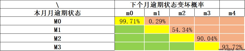
【 Performance period 】 The time point of the loan application ( namely : Observation points ) How long will it take to expose the performance , To thoroughly determine whether the customer is overdue . such as : After borrowing, I observed a customer after borrowing 60 The performance of those installments in the past few days is to repay on time , You can judge him to be good / Bad customer ?
This is to determine the performance period , The common analysis method is Vintage analysis (Vintage In the credit field, it can not only be used to evaluate the quality of customers, but also the time required for full exposure , That is, maturity , It can also be used to analyze the differences of risk control strategies in different periods ), By analyzing the increasing trend of historical cumulative bad user exposure , To determine at least how long it takes to fully expose most of the bad customers . The bad definition of the following example is M4+, We can see the M4+ Bad customers go through 9 perhaps 10 About months of performance , Basically, they can all be exposed , After that, the total number of bad customers is relatively stable . Here we can position the performance period 9 perhaps 10 Months ~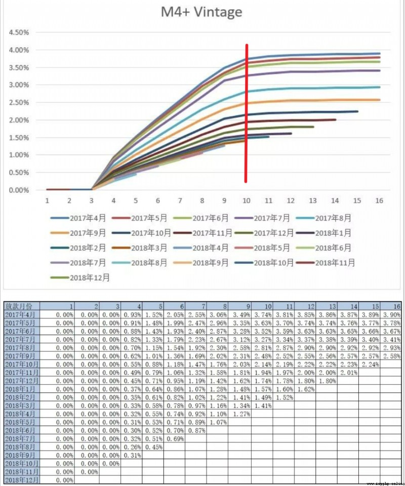
Determine the definition of bad and the required performance period , We can determine the label of the sample , The final delimited modeling sample :
Good user : Performance period ( Such as 9 Months ) There are no overdue user samples in .
Bad users : Performance period ( Such as 9 Months ) Overdue within ( Such as M2+) User samples for .
Grey user : There was overdue behavior during the performance period , But there is no bad definition ( Such as M2+) The sample of . notes : In practice, it is often only overdue 3 Users within days are also classified as good users .
For example, the present time is 2022-10 End of month , Performance period 9 For months , You can take 2022-01 Samples applied in and before the month ( This is also called Observation points ), Label it good or bad , modeling .
Through the introduction of credit scoring above , It's clear that good users are usually much larger than bad users , This is a typical scenario with extremely unbalanced categories , The treatment of imbalance is discussed below .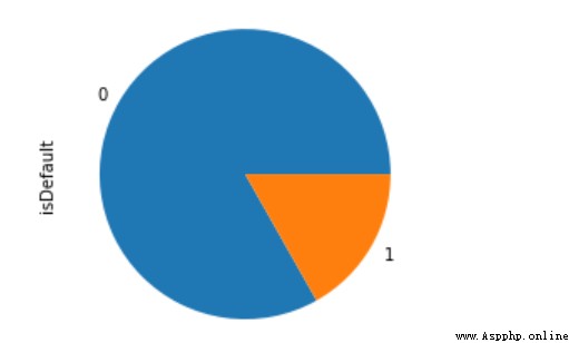
The data dictionary document for this dataset 、 Introduction to the competition and the code of this article , You can go to https://github.com/aialgorithm/Blog Download the corresponding code directory of the project
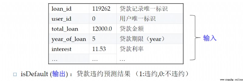
This data set is the personal loan default prediction data set of Zhongyuan bank , Some fields have been desensitized ( Most financial data are confidential ). The main characteristic fields are personal basic information 、 Economic capacity 、 Loan history information, etc  The data are 10000 Samples ,38 Primitive features of dimension , among isDefault Label , Whether it is overdue or not .

import pandas as pd
pd.set_option("display.max_columns",50)
train_bank = pd.read_csv('./train_public.csv')
print(train_bank.shape)
train_bank.head()
Data preprocessing is mainly for date information 、 The noise data is processed , And divide into the following categories 、 Characteristics of numeric types .
#  The date type :issueDate Convert to pandas The date type in , Process numerical characteristics
train_bank['issue_date'] = pd.to_datetime(train_bank['issue_date'])
#  Extract multi-scale features
train_bank['issue_date_y'] = train_bank['issue_date'].dt.year
train_bank['issue_date_m'] = train_bank['issue_date'].dt.month
#  Extraction time diff #  Convert to days
base_time = datetime.datetime.strptime('2000-01-01', '%Y-%m-%d')   #  Set the initial reference time randomly
train_bank['issue_date_diff'] = train_bank['issue_date'].apply(lambda x: x-base_time).dt.days
#  You can find earlies_credit_mon It should be the year - The format of the month , Here we simply extract the year
train_bank['earlies_credit_mon'] = train_bank['earlies_credit_mon'].map(lambda x:int(sorted(x.split('-'))[0]))
train_bank.head()
#  Working years treatment
train_bank['work_year'].fillna('10+ years', inplace=True)
work_year_map = {'10+ years': 10, '2 years': 2, '< 1 year': 0, '3 years': 3, '1 year': 1,
     '5 years': 5, '4 years': 4, '6 years': 6, '8 years': 8, '7 years': 7, '9 years': 9}
train_bank['work_year']  = train_bank['work_year'].map(work_year_map)
train_bank['class'] = train_bank['class'].map({'A': 0, 'B': 1, 'C': 2, 'D': 3, 'E': 4, 'F': 5, 'G': 6})
#  Missing value processing
train_bank = train_bank.fillna('9999')
#  distinguish   The number   Or category characteristics
drop_list = ['isDefault','earlies_credit_mon','loan_id','user_id','issue_date']
num_feas = []
cate_feas = []
for col in train_bank.columns:
    if col not in drop_list:
        try:
            train_bank[col] = pd.to_numeric(train_bank[col]) #  Convert to value
            num_feas.append(col)
        except:
            train_bank[col] = train_bank[col].astype('category')
            cate_feas.append(col)

print(cate_feas)
print(num_feas)If it is to use Lightgbm Modeling and forecasting default , Simple data processing , Basically, the code is over .lgb Tree model is a strong model of ensemble learning , Self contained absence 、 Processing of category variables , There is no need to do a lot of processing on the features , Modeling is very convenient , Models usually work well , You can also output the importance of the feature .
(By the way, Apply for the score card industry with logistic regression LR There will be more , Because the model is simple , The explanations are also quite good ).
def model_metrics(model, x, y):
    """  assessment  """
    yhat = model.predict(x)
    yprob = model.predict_proba(x)[:,1]
    fpr,tpr,_ = roc_curve(y, yprob,pos_label=1)
    metrics = {'AUC':auc(fpr, tpr),'KS':max(tpr-fpr),
               'f1':f1_score(y,yhat),'P':precision_score(y,yhat),'R':recall_score(y,yhat)}

    roc_auc = auc(fpr, tpr)
    plt.plot(fpr, tpr, 'k--', label='ROC (area = {0:.2f})'.format(roc_auc), lw=2)
    plt.xlim([-0.05, 1.05])  #  Set up x、y The upper and lower limits of the axis , So as not to coincide with the edge , Better observe the whole of the image
    plt.ylim([-0.05, 1.05])
    plt.xlabel('False Positive Rate')
    plt.ylabel('True Positive Rate')  #  Can use Chinese , But you need to import some libraries that are Fonts
    plt.title('ROC Curve')
    plt.legend(loc="lower right")
    return metrics
#  Divide the data set : Training set and test set
train_x, test_x, train_y, test_y = train_test_split(train_bank[num_feas + cate_feas], train_bank.isDefault,test_size=0.3, random_state=0)
#  Training models
lgb=lightgbm.LGBMClassifier(n_estimators=5,leaves=5, class_weight= 'balanced',metric = 'AUC')
lgb.fit(train_x, train_y)
print('train ',model_metrics(lgb,train_x, train_y))
print('test ',model_metrics(lgb,test_x,test_y))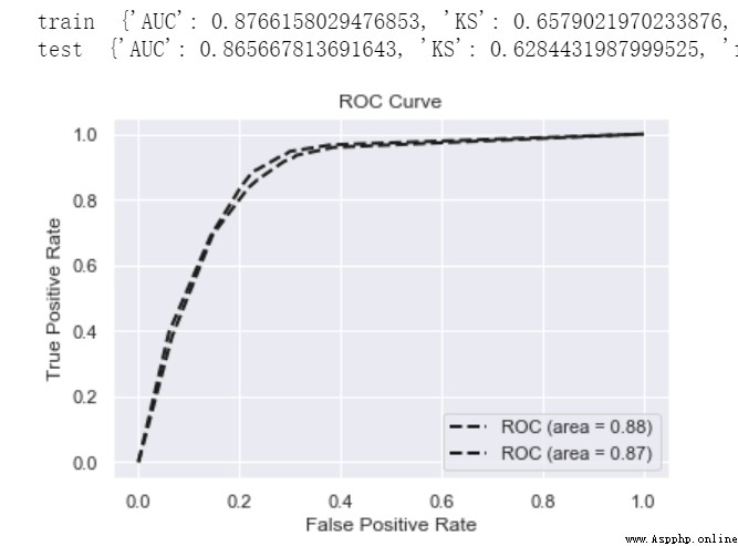
from lightgbm import plot_importance
plot_importance(lgb)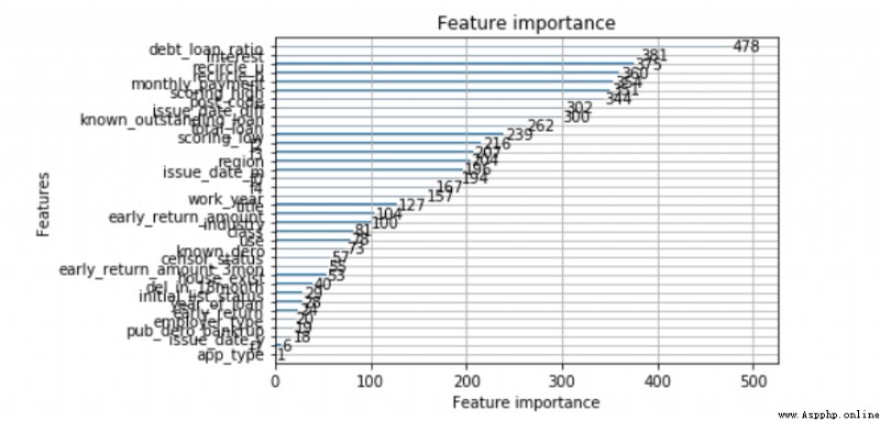
LR That's logical regression , It's a generalized linear model , Because its model is simple 、 Good explanation , It is the most commonly used in the financial industry .
And because LR Too simple , No non-linear capability , So we often need to use more complex feature engineering , For example, separate boxes WOE Coding method , Improve the nonlinear capability of the model . About LR Principle and optimization method of , It is highly recommended to read :
《 Comprehensively analyze and realize logical regression (Python)》
《 Summary of logistic regression optimization techniques ( whole )》
So let's go through toad Realize feature analysis 、 feature selection 、 Feature sub box and WOE code
#  data EDA analysis
toad.detector.detect(train_bank)
#  feature selection , According to relevance   Absence rate 、IV  Equal index
train_selected, dropped = toad.selection.select(train_bank,target = 'isDefault', empty = 0.5, iv = 0.05, corr = 0.7, return_drop=True, exclude=['earlies_credit_mon','loan_id','user_id','issue_date'])
print(dropped)
print(train_selected.shape)
#  Divide the training set   Test set
train_x, test_x, train_y, test_y = train_test_split(train_selected.drop(['loan_id','user_id','isDefault','issue_date','earlies_credit_mon'],axis=1), train_selected.isDefault,test_size=0.3, random_state=0)# Characteristic chi square boxes
combiner = toad.transform.Combiner()
# Train the data and specify the box dividing method
combiner.fit(pd.concat([train_x,train_y], axis=1), y='isDefault',method= 'chi',min_samples = 0.05,exclude=[])
# Save the sub box results in the form of Dictionary
bins = combiner.export()
bins Through the feature sub box , Each feature is discretized into individual sub boxes .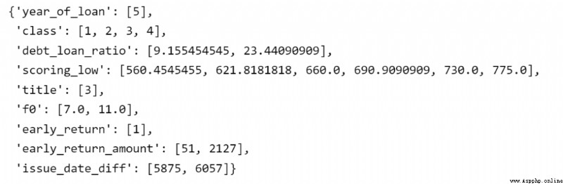
The next step is LR The characteristics of the feature engineering deal with -- Manually adjust the monotonicity of the sub box .
The significance of this step lies more in the business interpretive constraints of the features , The influence on the fitting effect of the model is not necessarily positive . Here we subjectively believe that the bad debt rates of different sub boxes with most characteristics badrate It should satisfy some monotonous relation , The ups and downs are not easy to understand . For example, the characteristic of credit inquiry times , It should be that the higher the value of the boxes , The higher the bad debt rate .( notes : For example, age characteristics may not satisfy this monotonic relationship )
We can check ebt_loan_ratio The distribution of this variable , according to bad_rate Trend chart , And ensure that the sample proportion of a single sub box is not less than 0.05, To adjust the distribution box , Achieve monotonicity .( Other features can be adjusted in this way , Monotonic adjustment is still time-consuming )
adj_var = 'scoring_low'
# The original sub box before adjustment  [560.4545455, 621.8181818, 660.0, 690.9090909, 730.0, 775.0]
adj_bin = {adj_var: [ 660.0, 700.9090909, 730.0, 775.0]}
c2 = toad.transform.Combiner()
c2.set_rules(adj_bin)
data_ = pd.concat([train_x,train_y], axis=1)
data_['type'] = 'train'
temp_data = c2.transform(data_[[adj_var,'isDefault','type']], labels=True)
from toad.plot import badrate_plot, proportion_plot
# badrate_plot(temp_data, target = 'isDefault', x = 'type', by = adj_var)
# proportion_plot(temp_data[adj_var])
from toad.plot import  bin_plot,badrate_plot
bin_plot(temp_data, target = 'isDefault',x=adj_var)
Before adjustment 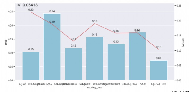
After the adjustment 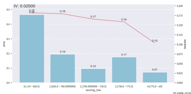
#  Update the adjusted sub box
combiner.set_rules(adj_bin)
combiner.export()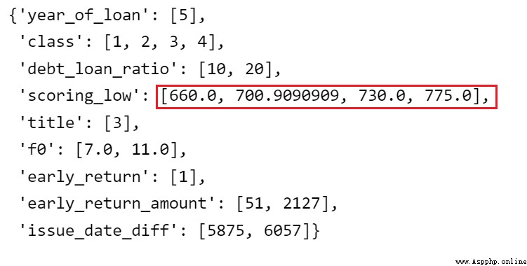
The next step is to do the sorting of each feature WOE code , adopt WOE Codes give different weights to each sub box , promote LR The nonlinearity of the model .
# Calculation WOE, Only in the training set WOE, Otherwise, the label will leak
transer = toad.transform.WOETransformer()
binned_data = combiner.transform(pd.concat([train_x,train_y], axis=1))
# Yes WOE The value of , Map to the original dataset . For training sets fit_transform, For the test set transform.
data_tr_woe = transer.fit_transform(binned_data, binned_data['isDefault'],  exclude=['isDefault'])
data_tr_woe.head()
## test woe
#  First, divide the boxes
binned_data = combiner.transform(test_x)
# Yes WOE The value of , Map to the original dataset . For the test set transform.
data_test_woe = transer.transform(binned_data)
data_test_woe.head()Use woe Encoding train Data training model . For the extremely unbalanced data set of financial risk control , A common approach is to do positive sampling of very few classes or use cost sensitive learning class_weight='balanced', To increase the learning weight of very few classes . so :《 Solve the sample imbalance in one article ( whole )》
about LR Equiweak model , Usually, we will find the difference between the training set and the test set (gap) It's less , That is, there is little over fitting phenomenon .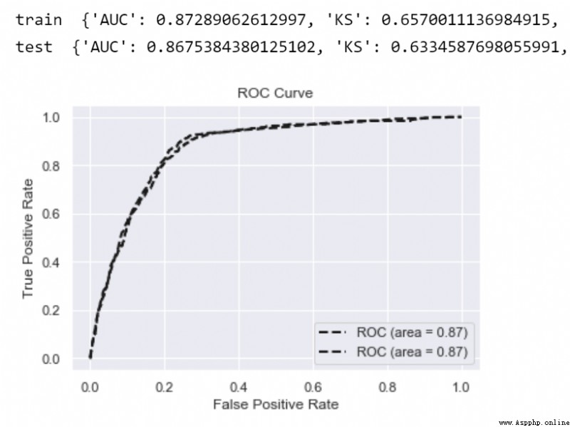
#  Training LR Model
from sklearn.linear_model import LogisticRegression
lr = LogisticRegression(class_weight='balanced')
lr.fit(data_tr_woe.drop(['isDefault'],axis=1), data_tr_woe['isDefault'])
print('train ',model_metrics(lr,data_tr_woe.drop(['isDefault'],axis=1), data_tr_woe['isDefault']))
print('test ',model_metrics(lr,data_test_woe,test_y))Use trained LR Model , Output ( probability ) Score distribution table , Combined with the manslaughter rate 、 Recall rates and business needs can determine an appropriate score threshold cutoff ( notes : In the real world , In general, probability nonlinearity is also transformed into a more intuitive integer fraction score=A-B*ln(odds), Convenient scorecard is more intuitive 、 Unified application .)
train_prob = lr.predict_proba(data_tr_woe.drop(['isDefault'],axis=1))[:,1]
test_prob = lr.predict_proba(data_test_woe)[:,1]
# Group the predicted scores in bins with same number of samples in each (i.e. "quantile" binning)
toad.metrics.KS_bucket(train_prob, data_tr_woe['isDefault'], bucket=10, method = 'quantile')
When the probability of predicting this user is greater than the set threshold , This means that the default probability of this user is very high , You can refuse his loan application .
 Past highlights
It is suitable for beginners to download the route and materials of artificial intelligence ( Image & Text + video ) Introduction to machine learning series download Chinese University Courses 《 machine learning 》( Huang haiguang keynote speaker ) Print materials such as machine learning and in-depth learning notes 《 Statistical learning method 》 Code reproduction album machine learning communication qq Group 955171419, Please scan the code to join wechat group