詳閉幕列表算法與其相干的C說話完成。本站提示廣大學習愛好者:(詳閉幕列表算法與其相干的C說話完成)文章只能為提供參考,不一定能成為您想要的結果。以下是詳閉幕列表算法與其相干的C說話完成正文
散列表(也叫哈希表)是一種查找算法,與鏈表、樹等算法分歧的是,散列表算法在查找時不須要停止一系列和症結字(症結字是數據元素中某個數據項的值,用以標識一個數據元素)的比擬操作。
散列表算法願望能盡可能做到不經由任何比擬,經由過程一次存取就可以獲得所查找的數據元素,因此必需要在數據元素的存儲地位和它的症結字(可用key表現)之間樹立一個肯定的對應關系,使每一個症結字和散列表中一個獨一的存儲地位絕對應。是以在查找時,只需依據這個對應關系找到給定症結字在散列表中的地位便可。這類對應關系被稱為散列函數(可用h(key)表現)。
依據設定的散列函數h(key)和處置抵觸的辦法將一組症結字key映像到一個無限的持續的地址區間上,並以症結字在地址區間中的像作為數據元素在表中的存儲地位,這類表便被稱為散列表,這一映像進程稱為散列,所得存儲地位稱為散列地址。
症結字、散列函數和散列表的關系以下圖所示:
1、散列函數
散列函數是從症結字到地址區間的映像。
好的散列函數可以或許使得症結字經由散列後獲得一個隨機的地址,以便使一組症結字的散列地址平均地散布在全部地址區間中,從而削減抵觸。
經常使用的結構散列函數的辦法有:
(1)、直接定址法
取症結字或症結字的某個線性函數值為散列地址,即:
h(key) = key 或 h(key) = a * key + b
個中a和b為常數。
(2)、數字剖析法
(3)、平方取值法
取症結字平方後的中央幾位為散列地址。
(4)、折疊法
將症結字朋分成位數雷同的幾部門(最初一部門的位數可以分歧),然後取這幾部門的疊加和(捨去進位)作為散列地址。
(5)、除留余數法
取症結字被某個不年夜於散列表表長m的數p除後所得的余數為散列地址,即:
h(key) = key MOD p p ≤ m
(6)、隨機數法
選擇一個隨機函數,取症結字的隨機函數值為它的散列地址,即:
h(key) = random(key)
個中random為隨機函數。
2、處置抵觸
對分歧的症結字能夠獲得統一散列地址,即key1 ≠ key2,而h(key1)= h(key2),這類景象稱為抵觸。具有雷同函數值的症結字對該散列函數來講稱作同義詞。
在普通情形下,散列函數是一個緊縮映像,這就弗成防止地會發生抵觸,是以,在創立散列表時不只要設定一個好的散列函數,並且還要設定一種處置抵觸的辦法。
經常使用的處置抵觸的辦法有:
(1)、開放定址法
hi =(h(key) + di) MOD m i =1,2,…,k(k ≤ m-1)
個中,h(key)為散列函數,m為散列表表長,di為增量序列,可有以下三種取法:
1)、di = 1,2,3,…,m-1,稱線性探測再散列;
2)、di = 12,-12,22,-22,32,…,±k2 (k ≤m/2),稱二次探測再散列;
3)、di = 偽隨機數序列,稱偽隨機探測再散列。
(2)、再散列法
hi = rhi(key) i = 1,2,…,k
rhi均是分歧的散列函數。
(3)、鏈地址法
將一切症結字為同義詞的數據元素存儲在統一線性鏈表中。假定某散列函數發生的散列地址在區間[0,m-1]上,則設立一個指針型向量void *vec[m],其每一個重量的初始狀況都是空指針。凡散列地址為i的數據元素都拔出到頭指針為vec[i]的鏈表中。在鏈表中的拔出地位可以在表頭或表尾,也能夠在表的中央,以堅持同義詞在統一線性鏈表中按症結字有序分列。
(4)、樹立一個公共溢出區
相干的C說話說明
hash.h
哈希表數據構造&&接口界說頭文件
  #ifndef HASH_H
  #define HASH_H

  #define HASH_TABLE_INIT_SIZE 7

  #define SUCCESS 1
  #define FAILED 0


  /**
   * 哈希表槽的數據構造
   */
  typedef struct Bucket {
    char *key;
    void *value;
    struct Bucket *next;
  } Bucket;

  /**
   * 哈希表數據構造
   */
  typedef struct HashTable {
    int size;  // 哈希表年夜小
    int elem_num;  // 哈希表曾經保留的數據元素個數
    Bucket **buckets;
  } HashTable;

  int hashIndex(HashTable *ht, char *key);
  int hashInit(HashTable *ht);
  int hashLookup(HashTable *ht, char *key, void **result);
  int hashInsert(HashTable *ht, char *key, void *value);
  int hashRemove(HashTable *ht, char *key);
  int hashDestory(HashTable *ht);
  #endif
hash.c
哈希表操作函數詳細完成
  #include <stdio.h>
  #include <stdlib.h>
  #include <string.h>
  #include "hash.h"

  /**
   * 初始化哈希表
   *
   * T = O(1)
   *
   */
  int hashInit(HashTable *ht)
  {
    ht->size = HASH_TABLE_INIT_SIZE;
    ht->elem_num = 0;
    ht->buckets = (Bucket **)calloc(ht->size, sizeof(Bucket *));

    if (ht->buckets == NULL)
      return FAILED;
    else
      return SUCCESS;
  }

  /**
   * 散列函數
   *
   * T = O(n)
   *
   */
  int hashIndex(HashTable *ht, char *key)
  {
    int hash = 0;

    while (*key != '\0') {
      hash += (int)*key;
      key ++;
    }

    return hash % ht->size;
  }

  /**
   * 哈希查找函數
   *
   * T = O(n)
   *
   */
  int hashLookup(HashTable *ht, char *key, void **result)
  {
    int index = hashIndex(ht, key);

    Bucket *bucket = ht->buckets[index];

    while (bucket) {
      if (strcmp(bucket->key, key) == 0) {
        *result = bucket->value;
        return SUCCESS;
      }
      bucket = bucket->next;
    }

    return FAILED;
  }


  /**
   * 哈希表拔出操作
   *
   * T = O(1)
   *
   */
  int hashInsert(HashTable *ht, char *key, void *value)
  {
    int index = hashIndex(ht, key);

    Bucket *org_bucket, *tmp_bucket;
    org_bucket = tmp_bucket = ht->buckets[index];

    // 檢討key能否曾經存在於hash表中
    while (tmp_bucket) {
      if (strcmp(tmp_bucket->key, key) == 0) {
        tmp_bucket->value = value;
        return SUCCESS;
      }
      tmp_bucket = tmp_bucket->next;
    }

    Bucket *new = (Bucket *)malloc(sizeof(Bucket));

    if (new == NULL)  return FAILED;

    new->key = key;
    new->value = value;
    new->next = NULL;

    ht->elem_num += 1;

    // 頭插法
    if (org_bucket) {
      new->next = org_bucket;
    }

    ht->buckets[index] = new;

    return SUCCESS;
  }

  /**
   * 哈希刪除函數
   *
   * T = O(n)
   *
   */
  int hashRemove(HashTable *ht, char *key)
  {
    int index = hashIndex(ht, key);

    Bucket *pre, *cur, *post;

    pre = NULL;
    cur = ht->buckets[index];

    while (cur) {
      if (strcmp(cur->key, key) == 0) {
        post = cur->next;

        if (pre == NULL) {
          ht->buckets[index] = post;
        } else {
          pre->next = post;
        }

        free(cur);

        return SUCCESS;
      }

      pre = cur;
      cur = cur->next;
    }

    return FAILED;
  }

  /**
   * 哈希表燒毀函數
   *
   * T = O(n)
   */
  int hashDestory(HashTable *ht)
  {
    int i;
    Bucket *cur, *tmp;

    cur = tmp = NULL;

    for (i = 0; i < ht->size; i ++) {
      cur = ht->buckets[i];

      while (cur) {
        tmp = cur->next;
        free(cur);
        cur = tmp;
      }
    }

    free(ht->buckets);

    return SUCCESS;
  }
test.c
單位測試文件
  #include <stdio.h>
  #include <stdlib.h>
  #include <string.h>
  #include <assert.h>
  #include "hash.h"

  int main(int argc, char **argv)
  {
    HashTable *ht = (HashTable *)malloc(sizeof(HashTable));
    int result = hashInit(ht);

    assert(result == SUCCESS);

    /* Data */
    int int1 = 10;
    int int2 = 20;
    char str1[] = "Hello World!";
    char str2[] = "Value";
    char str3[] = "Hello New World!";

    /* to find data container */
    int *j = NULL;
    char *find_str = NULL;

    /* Test Key Insert */
    printf("Key Insert:\n");
    hashInsert(ht, "FirInt", &int1);
    hashInsert(ht, "FirStr", str1);
    hashInsert(ht, "SecStr", str2);
    printf("Pass Insert\n");

    /* Test Key Lookup*/
    printf("Key Lookup:\n");
    result = hashLookup(ht, "FirStr", &find_str);
    assert(result == SUCCESS);
    printf("pass lookup, the value is %s\n", find_str);

    /* Test Update */
    printf("Key Update:\n");
    hashInsert(ht, "FirStr", str3);
    result = hashLookup(ht, "FirStr", &find_str);
    assert(result == SUCCESS);
    printf("pass update, the value is %s\n", find_str);

    return 0;
  }
編譯辦法
gcc -Wall -g -o main test.c hash.c
運轉成果
開放尋址法
在開放尋址法(open addressing)中,一切的元素都寄存在散列內外。亦即,每一個表項或包括靜態聚集的一個元素,或包括NIL。當查找一個元素時,要檢討一切的表項,直到找到所需的元素,或許終究發明該元素不在表中。不像在鏈接法中,這沒有鏈表,也沒有元素寄存在散列表外。在這類辦法中,散列表能夠會被填滿,乃至於不克不及拔出任何新的元素,但裝載因子a是相對不會跨越1的
線性探測法
第一次抵觸挪動1個單元,再次抵觸時,挪動2個,再次抵觸,挪動3個單元,依此類推
它的散列函數是:H(x) = (Hash(x) + F(i)) mod TableSize, 且F(0) = 0
舉例(騰訊面試標題)
已知一個線性表(38, 25, 74, 63, 52, 48),假定采取散列函數 h(key) = key % 7 盤算散列地址,並散列存儲在散列表 A[0..6]中,若采取線性探測辦法處理抵觸,則在該散列表長進行等幾率勝利查找的均勻長度為 ?
下邊模仿線性探測:
38 % 7 == 3, 無抵觸, ok
25 % 7 == 4, 無抵觸, ok
74 % 7 == 4, 抵觸, (4 + 1)% 7 == 5, 無抵觸,ok
63 % 7 == 0, 無抵觸, ok
52 % 7 == 3, 抵觸, (3 + 1) % 7 == 4. 抵觸, (4 + 1) % 7 == 5, 抵觸, (5 + 1)%7 == 6,無抵觸,ok
48 % 7 == 6, 抵觸, (6 + 1) % 7 == 0, 抵觸, (0 + 1) % 7 == 1,無抵觸,ok
繪圖以下:
均勻查找長度 = (1 + 3 + 1 + 1 + 2 + 3) % 6 = 2
線性探測辦法比擬輕易完成,但它卻存在一個成績,稱為一次群集(primary clustering).跟著時光的推移,持續被占用的槽赓續增長,均勻查找時光也跟著赓續增長。集群景象很輕易湧現,這是由於當一個空槽前有i個滿的槽時,該空槽為下一個將被占用的槽的幾率是 (i + 1) / n.持續占用的槽的序列會變得愈來愈長,因此均勻查找時光也會隨之增長
平方探測
為了不下面提到的一個群集的成績:第一次抵觸時挪動1(1的平方)個單元,再次抵觸時,挪動4(2的平方)個單元,還抵觸,挪動9個單元,依此類推。F(i) = i * i