本系列旨在記錄人工智能邊緣計算的基礎知識,共分為三部分:
OpenCV-python::圖像、視頻數據的處理、一些應用所需python工具包:
pip install numpy
pip install opencv-python
pip install matplotlib
import numpy as np
import cv2
import matplotlib.pyplot as plt
# 讀取圖片 彩色(默認) 1、灰色 0、帶alpha通道 -1
img = cv2.imread("img.png", 1)
cv2.imshow("img", img)
cv2.waitKey(0)
#打印圖片屬性
print(img.shape, img.size, img.type)
# 用plt顯示
plt.imshow(img[:100, :100, ::-1])
plt.title("plt顯示結果"), plt.xticks([]), plt.yticks([])
# 漢字防止出現亂碼
plt.rcParams['font.sans-serif']=['SimHei']
plt.rcParams['axes.unicode_minus'] = False
plt.show()
# 保存圖像
cv.imwrite('img_leftTop.png',img[:100, :100, :])
cv2顯示結果: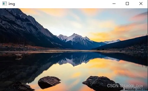
圖片屬性:
(281, 500, 3):對應(高、寬、通道)
421500 :281 * 500 * 3,數據量
uint8:無符號8bit整數
plt這裡截取了左上角一塊100*100的部分圖片,由於cv2讀取的圖片數據格式為BGR,所以對img數組的最後一維進行了倒置,顯示結果: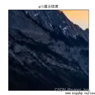
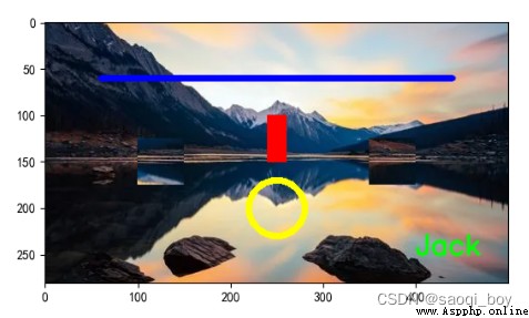
# 在img上畫一條從[60, 60]到[440,60]寬度為5的藍色(這裡是BGR)直線
cv2.line(img, [60, 60], [440, 60], [255, 0, 0], 5)
# 在img上畫一個從[240,100]到[260,150]的紅色實心矩形,當畫筆粗細為-1時畫實心圖形
cv2.rectangle(img, (240, 100), (260, 150), (0, 0, 255), -1)
# 在img上畫一個圓心為(250,200),半徑為30線條寬度為5的黃色空心圓
cv2.circle(img, [250, 200], 30, (0, 255, 255), 5)
# 在img上(250,450)位置寫上Jack,字體為cv2.FONT_HERSHEY_SIMPLEX,大小為 1,顏色為綠色,線條粗細為22,這裡不支持中文
cv2.putText(img, 'Jack', (400, 250), cv2.FONT_HERSHEY_SIMPLEX, 1, (0, 255, 0), 2, cv2.LINE_AA)
# 深拷貝
import copy
a = copy.deepcopy(img[125:175, 100:150, :])
# 交換兩個區域的部分圖片
img[125:175, 100:150, :] = img[125:175, 350:400, :]
img[125:175, 350:400, :] = a
# 將通道由BGR轉變為RGB
img = cv2.cvtColor(img, cv2.COLOR_BGR2RGB)
plt.imshow(img)
plt.show()
# 在img上填充凸多邊形
area1 = [[150, 80], [115, 160], [195, 160]]
# 填充單個
cv2.fillConvexPoly(img, np.array(area1), (0, 255, 0))
plt.imshow(img[:, :, ::-1])
plt.show()
area2 = [[350, 80], [305, 160], [395, 160]]
# 填充多個
cv2.fillPoly(img, [np.array(area1), np.array(area2)], (0, 0, 0))
plt.imshow(img[:, :, ::-1])
plt.show()
單個: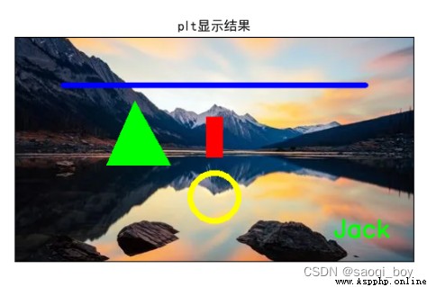
多個: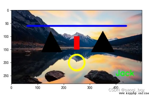
# 通道拆分
b,g,r = cv2.split(img)
print(b.shape)
b_img = np.zeros((281, 500, 3), np.uint8)
b_img[:, :, :1] = np.expand_dims(b, 2)
plt.imshow(b_img[:, :, ::-1])
plt.show()
g_img = np.zeros((281, 500, 3), np.uint8)
g_img[:, :, 1:2] = np.expand_dims(g, 2)
plt.imshow(g_img[:, :, ::-1])
plt.show()
r_img = np.zeros((281, 500, 3), np.uint8)
r_img[:, :, 2:3] = np.expand_dims(r, 2)
plt.imshow(r_img[:, :, ::-1])
plt.show()
# 通道合並
img = cv2.merge((b, g, r))
plt.imshow(img)
plt.show()
B: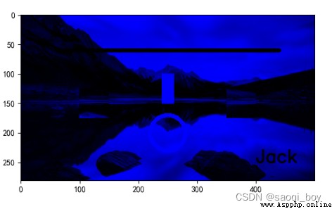
G: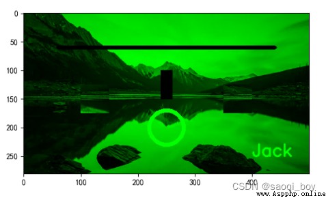
R: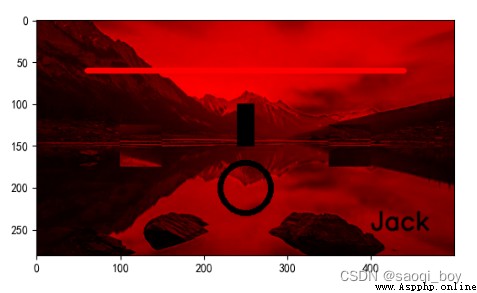
合並: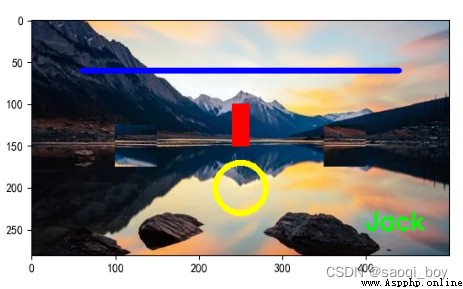
這裡需保證參與運算的圖片shape相等
img1 = cv2.imread("img_1.png")
img2 = cv2.imread("img_2.png")
plt.imshow(img1[:, :, ::-1])
plt.show()
plt.imshow(img2[:, :, ::-1])
plt.show()
img = cv2.add(img1, img2)
plt.imshow(img[:, :, ::-1])
plt.show()
img1原圖: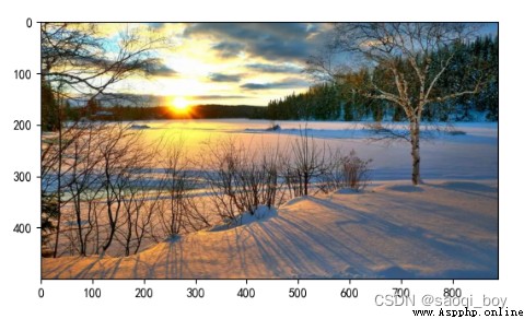
img2原圖: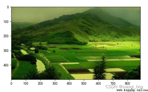
相加後:(當相加和大於255時取255)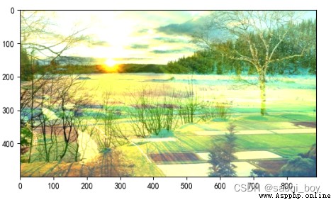
img1 = cv2.imread("img_1.png")
img2 = cv2.imread("img_2.png")
img = img1 + img2
plt.imshow(img[:, :, ::-1])
plt.show()
和超過255時取255余數: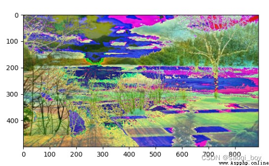
img = cv2.bitwise_and(img1, img2)
plt.imshow(img[:, :, ::-1])
plt.show()
1 & 1 = 1, 其他為0: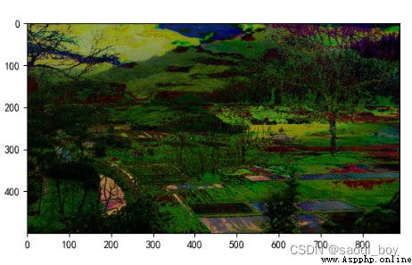
img = cv2.bitwise_or(img1, img2)
plt.imshow(img[:, :, ::-1])
plt.show()
** 0 | 0 = 0, 其他為1:**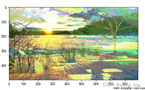
img = cv2.bitwise_xor(img1, img2)
plt.imshow(img[:, :, ::-1])
plt.show()
1 ^ 1, 0 ^ 0 為1,其他為0: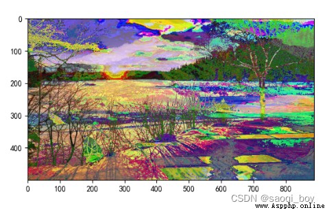
img = cv2.bitwise_not(img1)
plt.imshow(img[:, :, ::-1])
plt.show()
!x = 255 - x: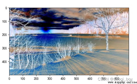
img = cv2.addWeighted(img1, 0.7, img2, 0.3, 0)
plt.imshow(img[:, :, ::-1])
plt.show()
0.7img+0.3img2+0: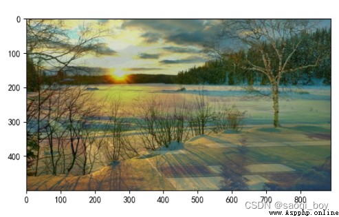
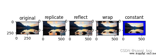
img = cv2.imread("img.png")
replicate = cv2.copyMakeBorder(img, 50, 50, 50, 50, cv2.BORDER_REPLICATE)
reflect = cv2.copyMakeBorder(img, 50, 50, 50, 50, cv2.BORDER_REFLECT_101)
wrap = cv2.copyMakeBorder(img, 50, 50, 50, 50, cv2.BORDER_WRAP)
constant = cv2.copyMakeBorder(img, 50, 50, 50, 50, cv2.BORDER_CONSTANT, value=(255, 0, 0))
plt.subplot(1, 5, 1), plt.imshow(img[:, :, ::-1]), plt.title("original")
plt.subplot(1, 5, 2), plt.imshow(replicate[:, :, ::-1]), plt.title("replicate")
plt.subplot(1, 5, 3), plt.imshow(reflect[:, :, ::-1]), plt.title("reflect")
plt.subplot(1, 5, 4), plt.imshow(wrap[:, :, ::-1]), plt.title("wrap")
plt.subplot(1, 5, 5), plt.imshow(constant[:, :, ::-1]), plt.title("constant")
plt.show()
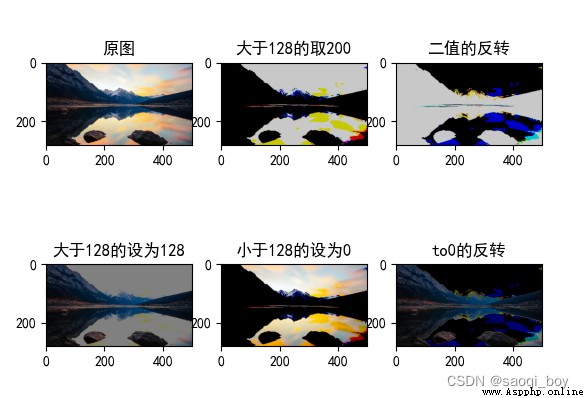
# 阈值處理
_, thresh1 = cv2.threshold(img, 128, 200, cv2.THRESH_BINARY)
_, thresh2 = cv2.threshold(img, 128, 200, cv2.THRESH_BINARY_INV)
_, thresh3 = cv2.threshold(img, 128, 200, cv2.THRESH_TRUNC)
_, thresh4 = cv2.threshold(img, 128, 200, cv2.THRESH_TOZERO)
_, thresh5 = cv2.threshold(img, 128, 200, cv2.THRESH_TOZERO_INV)
plt.subplot(2, 3, 1), plt.imshow(img[:, :, ::-1]), plt.title("原圖")
plt.subplot(2, 3, 2), plt.imshow(thresh1[:, :, ::-1]), plt.title("大於128的取200")
plt.subplot(2, 3, 3), plt.imshow(thresh2[:, :, ::-1]), plt.title("二值的反轉")
plt.subplot(2, 3, 4), plt.imshow(thresh3[:, :, ::-1]), plt.title("大於128的設為128")
plt.subplot(2, 3, 5), plt.imshow(thresh4[:, :, ::-1]), plt.title("小於128的設為0")
plt.subplot(2, 3, 6), plt.imshow(thresh5[:, :, ::-1]), plt.title("to0的反轉")
plt.rcParams['font.sans-serif']=['SimHei']#漢字防止出現亂碼
plt.rcParams['axes.unicode_minus'] = False
plt.show()
img = cv2.imread("img.png")
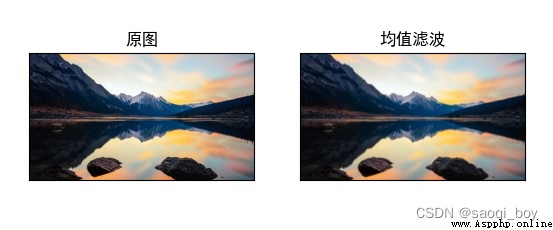
# 均值濾波
img_average = cv2.blur(img, (3, 3))
plt.subplot(1, 2, 1), plt.imshow(img[:, :, ::-1]), plt.title("原圖"), plt.xticks([]), plt.yticks([])
plt.subplot(1, 2, 2), plt.imshow(img_average[:, :, ::-1]), plt.title("均值濾波"), plt.xticks([]), plt.yticks([])
plt.rcParams["font.sans-serif"] = ["SimHei"]
plt.rcParams['axes.unicode_minus'] = False
plt.show()
img_box = cv2.boxFilter(img, -1, (5, 5), normalize=False)
plt.subplot(1, 2, 1), plt.imshow(img[:, :, ::-1]), plt.title("原圖"), plt.xticks([]), plt.yticks([])
plt.subplot(1, 2, 2), plt.imshow(img_box[:, :, ::-1]), plt.title("方框濾波-未求均值"), plt.xticks([]), plt.yticks([])
plt.rcParams["font.sans-serif"] = ["SimHei"]
plt.rcParams['axes.unicode_minus'] = False
plt.show()
當normal為true時與均值濾波相同,當為false時不取均值,和大於255的取255: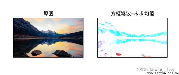
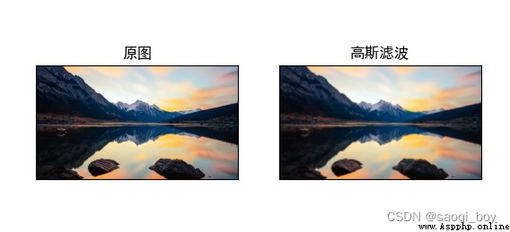
img_gauss = cv2.GaussianBlur(img, (5, 5), 1)
plt.subplot(1, 2, 1), plt.imshow(img[:, :, ::-1]), plt.title("原圖"), plt.xticks([]), plt.yticks([])
plt.subplot(1, 2, 2), plt.imshow(img_gauss[:, :, ::-1]), plt.title("高斯濾波"), plt.xticks([]), plt.yticks([])
plt.rcParams["font.sans-serif"] = ["SimHei"]
plt.rcParams['axes.unicode_minus'] = False
plt.show()
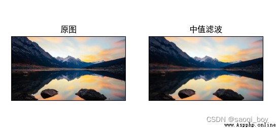
img_median = cv2.medianBlur(img, 5)
plt.subplot(1, 2, 1), plt.imshow(img[:, :, ::-1]), plt.title("原圖"), plt.xticks([]), plt.yticks([])
plt.subplot(1, 2, 2), plt.imshow(img_median[:, :, ::-1]), plt.title("中值濾波"), plt.xticks([]), plt.yticks([])
plt.rcParams["font.sans-serif"] = ["SimHei"]
plt.rcParams['axes.unicode_minus'] = False
plt.show()
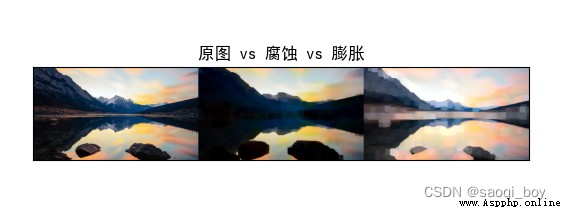
kernel = np.ones((3, 3), np.uint8)
img_erosion = cv2.erode(img, kernel, iterations=8)
img_dilate = cv2.dilate(img, kernel, iterations=8)
# 水平拼接
pk = np.hstack((img, img_erosion, img_dilate))
plt.imshow(pk[:, :, ::-1]), plt.title("原圖 vs 腐蝕 vs 膨脹"), plt.xticks([]), plt.yticks([])
plt.rcParams["font.sans-serif"] = ["SimHei"]
plt.rcParams['axes.unicode_minus'] = False
plt.show()
img_erosion = cv2.erode(img, kernel, iterations=1)
img_dilate = cv2.dilate(img, kernel, iterations=1)
td = img_dilate - img_erosion
gradient = cv2.morphologyEx(img, cv2.MORPH_GRADIENT, kernel)
pk = np.hstack((td, gradient))
plt.imshow(pk[:, :, ::-1]), plt.title("梯度運算:膨脹-腐蝕 vs gradient"), plt.xticks([]), plt.yticks([])
plt.rcParams["font.sans-serif"] = ["SimHei"]
plt.rcParams['axes.unicode_minus'] = False
plt.show()

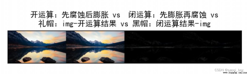
img_open = cv2.morphologyEx(img, cv2.MORPH_OPEN, kernel)
img_close = cv2.morphologyEx(img, cv2.MORPH_CLOSE, kernel)
img_limao = cv2.morphologyEx(img, cv2.MORPH_TOPHAT, kernel)
img_heimao = cv2.morphologyEx(img, cv2.MORPH_BLACKHAT, kernel)
pk = np.hstack((img_open, img_close, img_limao, img_heimao))
plt.imshow(pk[:, :, ::-1])
plt.title("開運算:先腐蝕後膨脹 vs 閉運算:先膨脹再腐蝕 vs\n"
"禮帽:img-開運算結果 vs 黑帽:img-閉運算結果"), plt.xticks([]), plt.yticks([])
plt.rcParams["font.sans-serif"] = ["SimHei"]
plt.rcParams['axes.unicode_minus'] = False
plt.show()
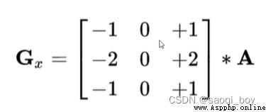
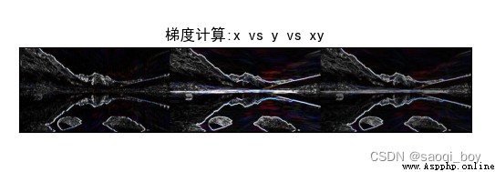
sobel_x = cv2.Sobel(img, cv2.CV_64F, 1, 0, ksize=3)
# 取結果的絕對值
sobel_x = cv2.convertScaleAbs(sobel_x)
sobel_y = cv2.Sobel(img, cv2.CV_64F, 0, 1, ksize=3)
sobel_y = cv2.convertScaleAbs(sobel_y)
sobel_xy = cv2.addWeighted(sobel_x, 0.5, sobel_y, 0.5, 0)
pk = np.hstack((sobel_x, sobel_y, sobel_xy))
plt.imshow(pk)
plt.title("梯度計算:x vs y vs xy"), plt.xticks([]), plt.yticks([])
plt.rcParams["font.sans-serif"] = ["SimHei"]
plt.rcParams['axes.unicode_minus'] = False
plt.show()
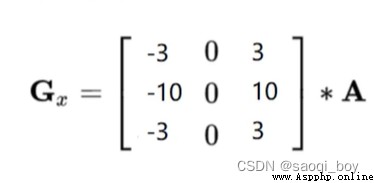
scharr_x = cv2.Scharr(img, cv2.CV_64F, 1, 0)
scharr_x = cv2.convertScaleAbs(scharr_x)
scharr_y = cv2.Scharr(img, cv2.CV_64F, 0, 1, ksize=3)
scharr_y = cv2.convertScaleAbs(scharr_y)
scharr_xy = cv2.addWeighted(scharr_x, 0.5, scharr_y, 0.5, 0)
plt.imshow(scharr_xy)
plt.title("scharr算子"), plt.xticks([]), plt.yticks([])
plt.rcParams["font.sans-serif"] = ["SimHei"]
plt.rcParams['axes.unicode_minus'] = False
plt.show()
比sobel算子效果更明顯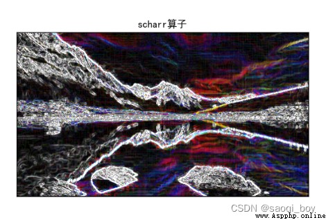
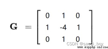
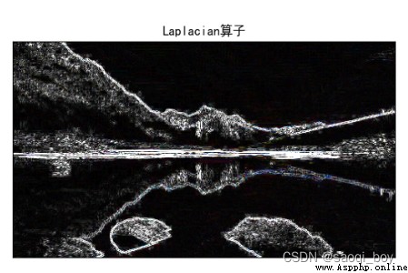
Laplacian = cv2.Laplacian(img, cv2.CV_64F, ksize=3)
Laplacian = cv2.convertScaleAbs(Laplacian)
plt.imshow(Laplacian)
plt.title("Laplacian算子"), plt.xticks([]), plt.yticks([])
plt.rcParams["font.sans-serif"] = ["SimHei"]
plt.rcParams['axes.unicode_minus'] = False
plt.show()
img_candy = cv2.Canny(img, 50, 100)
plt.imshow(img_candy), plt.title("candy"),plt.xticks([]), plt.yticks([])
plt.rcParams["font.sans-serif"] = ["SimHei"]
plt.rcParams['axes.unicode_minus'] = False
plt.show()
大致流程: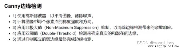
這裡使用的雙阈值為(50,100),阈值越小細節越多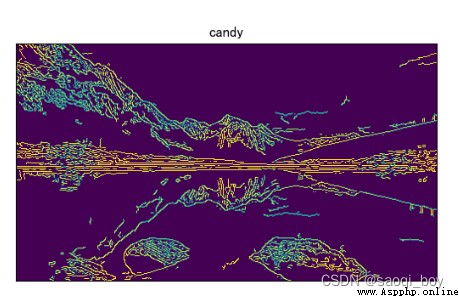
上采樣和下采樣:
img = cv2.imread("img_3.png")
print("img:", img.shape)
img1 = cv2.pyrDown(img)
print("img1:", img1.shape)
img2 = cv2.pyrUp(img)
print("img2:", img2.shape)
這裡是用的高斯內核卷積,放大或縮小2倍,運行結果:
img: (313, 500, 3)
img1: (157, 250, 3)
img2: (626, 1000, 3)
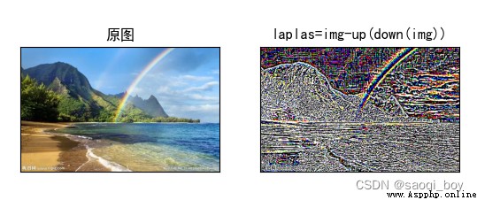
拉普拉斯計算:
laplas = img- cv2.pyrUp(cv2.pyrDown(img))[:313]
plt.subplot(1, 2, 1), plt.imshow(img[:, :, ::-1]), plt.title("原圖")
plt.xticks([]), plt.yticks([])
plt.subplot(1, 2, 2), plt.imshow(laplas[:, :, ::-1]), plt.title("laplas=img-up(down(img))")
plt.xticks([]), plt.yticks([])
plt.rcParams["font.sans-serif"] = ["SimHei"]
plt.rcParams["axes.unicode_minus"] = False
plt.show()
img = cv2.imread("img_2.png")
# 預處理
img_gray = cv2.cvtColor(img, cv2.COLOR_BGR2GRAY)
_, thresh = cv2.threshold(img_gray, 127, 255, cv2.THRESH_BINARY)
contours, hierarchy = cv2.findContours(thresh, cv2.RETR_TREE, cv2.CHAIN_APPROX_NONE)
# drawContours會改變原圖,所以這裡復制一份
img_draw = img.copy()
img_draw = cv2.drawContours(img_draw, contours, -1, (0, 0, 255), 2)
pk = np.hstack((img, img_draw))
plt.imshow(pk[:, :, ::-1]), plt.xticks([]), plt.yticks([]),
plt.show()
con = contours[300]
# 邊界矩形
x, y, w, h = cv2.boundingRect(con)
img_rect = cv2.rectangle(img, (x, y), (x+w, y+h), (0, 0, 255), 2)
plt.imshow(img_rect[:, :, ::-1]), plt.xticks([]), plt.yticks([]),
plt.show()
(x, y), radius = cv2.minEnclosingCircle(con)
img_circle = cv2.circle(img, (int(x), int(y)), int(radius), (0, 0, 255), 2)
plt.imshow(img_circle[:, :, ::-1]), plt.xticks([]), plt.yticks([]),
plt.show()
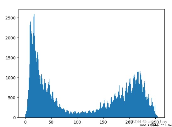
img = cv2.imread("img.png", 0)
# 直方圖統計
hist = cv2.calcHist([img], [0], None, [256], [0, 256])
print(hist.shape)
plt.hist(img.ravel(), 256)
plt.show()
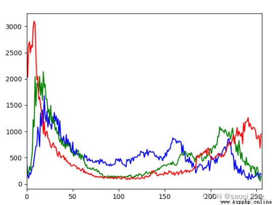
# 彩色直方圖
hist1 = cv2.calcHist([img], [0], None, [256], [0, 256])
plt.plot(hist1, color='b'), plt.xlim([0, 256])
hist2 = cv2.calcHist([img], [1], None, [256], [0, 256])
plt.plot(hist2, color='g'), plt.xlim([0, 256])
hist3 = cv2.calcHist([img], [2], None, [256], [0, 256])
plt.plot(hist3, color='r'), plt.xlim([0, 256])
plt.show()
img = cv2.imread("img.png", 0)
mask = np.zeros(img.shape[:2], np.uint8)
mask[50:250, 100:400] = 255
img_masked = cv2.bitwise_and(img, mask)
plt.imshow(img_masked, "gray"), plt.xticks([]), plt.yticks([])
plt.show()
hist = cv2.calcHist([img], [0], mask, [256], [0, 256])
plt.plot(hist), plt.xlim([0, 256])
plt.show()
添加mask後的圖片: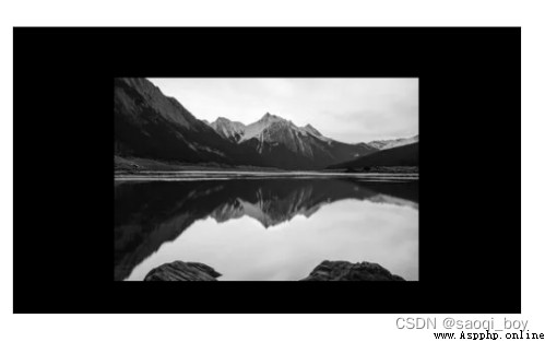
掩碼後的圖像像素直方圖: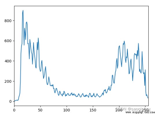
各個像數值從小到大的累積概率 * 255取整
img_equal = cv2.equalizeHist(img)
plt.hist(img_equal.ravel(), 256)
plt.show()
pk = np.hstack((img, img_equal))
plt.imshow(pk, "gray"), plt.xticks([]), plt.yticks([])
plt.show()
均衡化後的直方圖;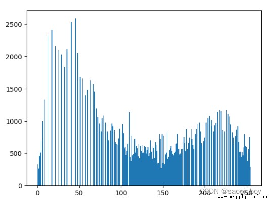
均衡化後的圖像對比,均衡化後的圖片(右)明顯更亮: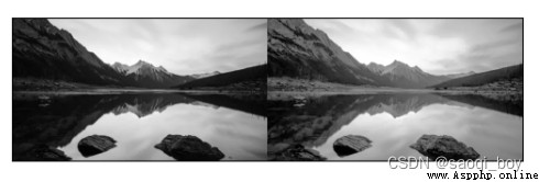
clahe = cv2.createCLAHE(clipLimit=2.0, tileGridSize=(8, 8))
img_clahe = clahe.apply(img)
pk = np.hstack((img, img_clahe))
plt.imshow(pk, "gray"), plt.xticks([]), plt.yticks([])
plt.show()
將圖像分成8 * 8份,分別進行均衡化後拼接到一起,連接處插值處理,相比於整體的均衡化,保留了更多細節: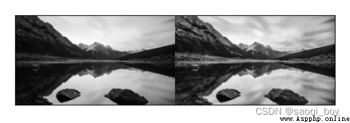
img = cv2.imread("img.png", 0)
img_f32 = np.float32(img)
dft = cv2.dft(img_f32, flags=cv2.DFT_COMPLEX_OUTPUT)
dft_shift = np.fft.fftshift(dft)
# 將數值放大到0~255
dft_magnitude = 20 * np.log(cv2.magnitude(dft_shift[:, :, 0], dft_shift[:, :, 1]))
plt.subplot(121), plt.imshow(img, "gray"), plt.title("img"), plt.xticks([]), plt.yticks([])
plt.subplot(122), plt.imshow(dft_magnitude, "gray"), plt.title("dft_magnitude"), plt.xticks([]), plt.yticks([])
plt.show()
rows, cols = img.shape
center_x, center_y = int(cols/2), int(rows/2)
# 低通濾波,使圖像模糊
mask = np.zeros((rows, cols, 2), np.uint8)
mask[center_y-30:center_y+30, center_x-30:center_x+30] = 1
# 傅裡葉反變換
f_shift = dft_shift * mask
f_ishift = np.fft.ifftshift(f_shift)
img_trans = cv2.idft(f_ishift)
img_trans = cv2.magnitude(img_trans[:, :, 0], img_trans[:, :, 1])
plt.subplot(121), plt.imshow(img, "gray"), plt.title("img"), plt.xticks([]), plt.yticks([])
plt.subplot(122), plt.imshow(img_trans, "gray"), plt.title("img_trans"), plt.xticks([]), plt.yticks([])
plt.show()
# 高通濾波,保留細節
mask = np.ones((rows, cols, 2), np.uint8)
mask[center_y-30:center_y+30, center_x-30:center_x+30] = 0
f_shift = dft_shift * mask
f_ishift = np.fft.ifftshift(f_shift)
img_trans = cv2.idft(f_ishift)
img_trans = cv2.magnitude(img_trans[:, :, 0], img_trans[:, :, 1])
plt.subplot(121), plt.imshow(img, "gray"), plt.title("img"), plt.xticks([]), plt.yticks([])
plt.subplot(122), plt.imshow(img_trans, "gray"), plt.title("img_trans"), plt.xticks([]), plt.yticks([])
plt.show()
原圖與空間頻域圖對比: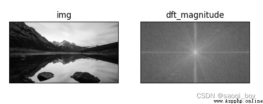
原圖與低通濾波對比: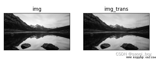
原圖與高通濾波對比: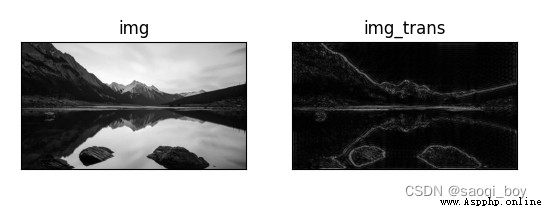
import cv2
# 讀取圖像
video = cv2.VideoCapture()
if not video.open("my_map.mp4"):
print("can not open the video")
exit(1)
else:
print("幀率:", video.get(cv2.CAP_PROP_FPS)) # cv2.CAP_PROP_FPS==5
print("幀數:", video.get(cv2.CAP_PROP_FRAME_COUNT)) # cv2.CAP_PROP_FRAME_COUNT==7
print("寬:", video.get(cv2.CAP_PROP_FRAME_WIDTH), "高:", video.get(cv2.CAP_PROP_FRAME_HEIGHT))
# 按幀讀取視頻
count = 0
while video.isOpened(): # 當視頻被打開時:
success, frame = video.read() # 讀取視頻,讀取到的某一幀存儲到frame,若是讀取成功,ret為True,反之為False
if success: # 若是讀取成功
count += 1
cv2.putText(frame, str(count)+"th", (20, 150), cv2.FONT_HERSHEY_DUPLEX, 0.9,
(147, 58, 31), 1)
cv2.imshow('frame', frame) # 顯示讀取到的這一幀畫面
key = cv2.waitKey(25) # 等待一段時間,並且檢測鍵盤輸入
if key == ord('s'): # 若是鍵盤輸入's',則保存當前幀
cv2.imwrite(str(count)+".jpg", frame)
if key == ord('q'): # 若是鍵盤輸入'q',則退出,釋放視頻
video.release() # 釋放視頻
break
else:
video.release()
cv2.destroyAllWindows() # 關閉所有窗口
print(count)
# 打開攝像頭
cap = cv2.VideoCapture(0)
fourcc = cv2.VideoWriter_fourcc(*'mp4v')
size = (int(cap.get(cv2.CAP_PROP_FRAME_WIDTH)), int(cap.get(cv2.CAP_PROP_FRAME_HEIGHT)))
# 創建VideoWriter
out = cv2.VideoWriter('camera.mp4', fourcc, cap.get(5), size)
# 按幀讀取視頻
count = 0
while cap.isOpened(): # 當視頻被打開時:
success, frame = cap.read() # 讀取視頻,讀取到的某一幀存儲到frame,若是讀取成功,ret為True,反之為False
# 翻轉
frame = cv2.flip(frame, 1)
if success: # 若是讀取成功
count += 1
# 寫入視頻
out.write(frame)
cv2.putText(frame, str(count)+"th", (20, 150), cv2.FONT_HERSHEY_DUPLEX, 0.9,
(147, 58, 31), 1)
cv2.imshow('frame', frame) # 顯示讀取到的這一幀畫面
key = cv2.waitKey(25) # 等待一段時間,並且檢測鍵盤輸入
if key == ord('q'): # 若是鍵盤輸入'q',則退出,釋放視頻
cap.release() # 釋放視頻
break
else:
cap.release()
out.release()
cv2.destroyAllWindows() # 關閉所有窗口
print(count)
第495幀的圖像: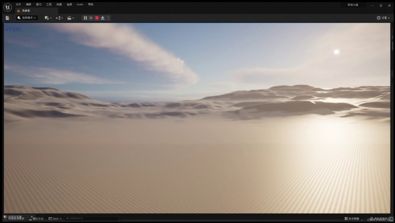
攝像頭錄制保存成功:
這裡識別主要是利用最外邊的大框將圖片轉正,然後用tesseract進行ocr識別,特殊情況需特殊處理,這裡僅針對這種含有外邊框的特殊情況,進行其他圖片的識別可能結果並不是很好。
tesseract下載地址:https://digi.bib.uni-mannheim.de/tesseract/
tesseract的git地址:https://github.com/tesseract-ocr/tesseract/
安裝tesseract後需要在所在環境pip install pytesseract
然後在python環境的site-packages包中找到pytesseract.py,更改其中的tesseract為絕對路徑: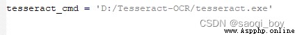
然後需以管理員身份運行pycharm。
import numpy as np
import cv2
import argparse
ap = argparse.ArgumentParser()
ap.add_argument("-i", "--image", required=True, help="掃描圖像的路徑")
args = vars(ap.parse_args())
print(args)
def order_points(pts):
rect = np.zeros((4, 2), dtype="float32")
s = pts.sum(axis=1)
rect[0] = pts[np.argmin(s)]
rect[2] = pts[np.argmax(s)]
diff = np.diff(pts, axis=1)
rect[1] = pts[np.argmin(diff)]
rect[3] = pts[np.argmax(diff)]
return rect
def four_points_transform(image, pts):
rect = order_points(pts)
(tl, tr, br, bl) = rect
widthA = np.sqrt(((br[0] - bl[0]) ** 2) + ((br[1] - bl[1]) ** 2))
widthB = np.sqrt(((tr[0] - tl[0]) ** 2) + ((tr[1] - tl[1]) ** 2))
max_width = max(int(widthA), int(widthB))
heightA = np.sqrt(((tr[0] - br[0]) ** 2) + ((tr[1] - br[1]) ** 2))
heightB = np.sqrt(((tl[0] - bl[0]) ** 2) + ((tl[1] - bl[1]) ** 2))
max_height = max(int(heightA), int(heightB))
dst = np.array([
[0, 0],
[max_width - 1, 0],
[max_width - 1, max_height - 1],
[0, max_height - 1]
], dtype="float32")
M = cv2.getPerspectiveTransform(rect, dst)
wraped = cv2.warpPerspective(image, M, (max_width, max_height))
return wraped
def resize(image, width=None, height=None, inter=cv2.INTER_AREA):
dim = None
(h, w) = image.shape[:2]
if width is None and height is None:
return image
if width is None:
r = height / float(h)
dim = (int(w * r), height)
else:
r = width / float(w)
dim = (width, int(h * r))
resized = cv2.resize(image, dim, interpolation=inter)
return resized
img = cv2.imread(args["image"])
ratio = img.shape[0] / 1000.0
orig = img.copy()
img = resize(orig, height=1000)
gray = cv2.cvtColor(img, cv2.COLOR_BGR2GRAY)
# 高斯濾波去除噪音點
gray = cv2.GaussianBlur(gray, (5, 5), 0)
# 邊緣檢測
edged = cv2.Canny(gray, 75, 200)
cv2.imshow("image", img)
cv2.imshow("edge", edged)
cv2.waitKey(0)
cv2.destroyAllWindows()
# 輪廓檢測
cnts = cv2.findContours(edged.copy(), cv2.RETR_LIST, cv2.CHAIN_APPROX_SIMPLE)[0]
cnts = sorted(cnts, key=cv2.contourArea, reverse=True)[:5]
# 遍歷輪廓
for c in cnts:
# 計算輪廓周長
peri = cv2.arcLength(c, True)
# 為輪廓近似外接化
approx = cv2.approxPolyDP(c, 0.02 * peri, True)
if len(approx) == 4:
screenCnt = approx
break
cv2.drawContours(img, [screenCnt], -1, (255, 0, 0), 2)
cv2.imshow("lined", img)
cv2.waitKey(0)
cv2.destroyAllWindows()
warped = four_points_transform(orig, screenCnt.reshape(4, 2) * ratio)
warped = cv2.cvtColor(warped, cv2.COLOR_BGR2GRAY)
cv2.imshow("warped", warped)
cv2.waitKey(0)
cv2.destroyAllWindows()
cv2.imwrite("scan.jpg", warped)
import pytesseract
from PIL import Image
text = pytesseract.image_to_string(Image.open("scan.jpg"))
print(text)
原圖: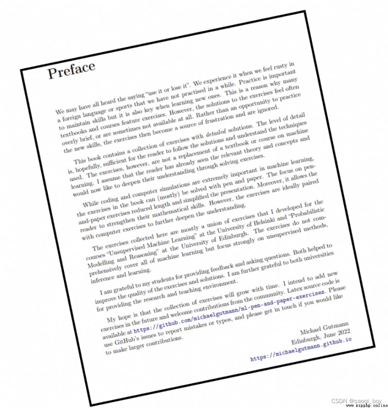
邊緣檢測: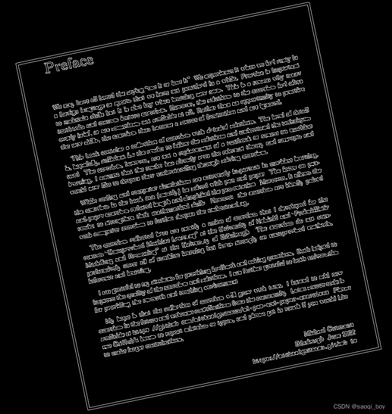
輪廓檢測,最大的輪廓:
圖像轉換:
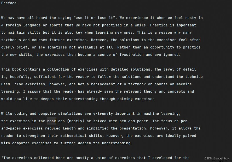
ocr文字識別結果,識別結果有些許瑕疵,但整體效果還不錯:
import cv2
img = cv2.imread("img_1.png")
gray = cv2.cvtColor(img, cv2.COLOR_BGR2GRAY)
dst = cv2.cornerHarris(gray, 2, 3, 0.04)
img[dst > 0.05*dst.max()] = [0, 0, 255]
cv2.imshow("corner", img)
cv2.waitKey(0)
cv2.destroyAllWindows()
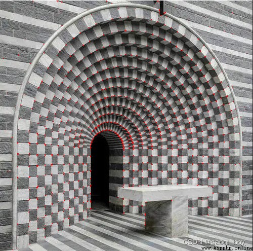
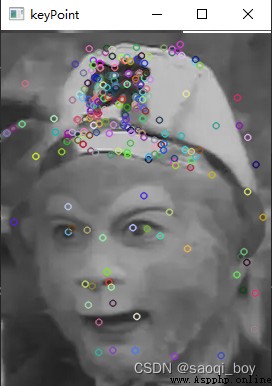
用sift函數獲取關鍵點:
img = cv2.imread("img_2.png")
gray = cv2.cvtColor(img, cv2.COLOR_BGR2GRAY)
sift = cv2.SIFT_create()
kp = sift.detect(gray, None)
img = cv2.drawKeypoints(gray, kp, img)
cv2.imshow("keyPoint", img)
cv2.waitKey(0)
cv2.destroyAllWindows()
匹配特征相似的關鍵點:
img1 = cv2.imread("img_2.png")
img2 = cv2.imread("img_3.png")
gray1 = cv2.cvtColor(img1, cv2.COLOR_BGR2GRAY)
gray2 = cv2.cvtColor(img2, cv2.COLOR_BGR2GRAY)
sift = cv2.SIFT_create()
keypoint1, descriptors1 = sift.detectAndCompute(gray1, None)
keypoint2, descriptors2 = sift.detectAndCompute(gray2, None)
# 蠻力匹配,計算特征向量歐式距離
bf = cv2.BFMatcher(crossCheck=True)
match = bf.match(descriptors1, descriptors2)
match = sorted(match, key=lambda x: x.distance)
img = cv2.drawMatches(gray1, keypoint1, gray2, keypoint2, match[-20:], None, flags=2)
cv2.imshow("match", img)
cv2.waitKey(0)
cv2.destroyAllWindows()
#k對最佳匹配, 1個點匹配多個,由k決定
bf = cv2.BFMatcher()
match = bf.knnMatch(descriptors1, descriptors2, k=2)
good = []
for m, n in match:
if m.distance < 0.75 * n.distance:
good.append(m)
good = np.expand_dims(good, 1)
img = cv2.drawMatchesKnn(gray1, keypoint1, gray2, keypoint2, good[:20], None, flags=2)
cv2.imshow("knn_match", img)
cv2.waitKey(0)
cv2.destroyAllWindows()
蠻力匹配: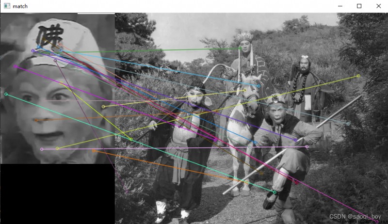
k對最佳匹配: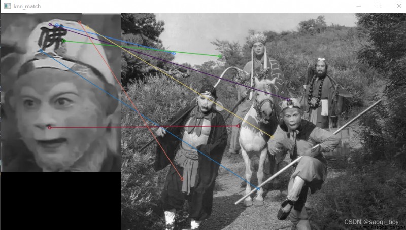
圖像拼接:
# 圖像拼接
MIN_MATCH_COUNT = 10
imgA, imgB = cv2.imread("img_4.jpg"), cv2.imread("img_5.jpg")
sift = cv2.SIFT_create()
(kpsA, featuresA), (kpsB, featuresB) = sift.detectAndCompute(imgA, None), sift.detectAndCompute(imgB, None)
matcher = cv2.BFMatcher()
good = []
matches = matcher.knnMatch(featuresB, featuresA, k=2)
for m, n in matches:
if m.distance < n.distance * 0.75:
good.append(m)
good1 = np.expand_dims(good, 1)
matching = cv2.drawMatchesKnn(imgA, kpsA, imgB, kpsB, good1[:20], None, matchColor=(0, 255, 0), flags=2)
if len(good) > MIN_MATCH_COUNT:
src_pts = np.float32([kpsB[m.queryIdx].pt for m in good]).reshape(-1, 1, 2)
dst_pts = np.float32([kpsA[m.trainIdx].pt for m in good]).reshape(-1, 1, 2)
# 求轉置矩陣
H, mask = cv2.findHomography(src_pts, dst_pts, cv2.RANSAC, 5.0)
# 求B轉變後的圖像
wrap = cv2.warpPerspective(imgB, H, (imgB.shape[1] + imgB.shape[1], imgB.shape[0] + imgB.shape[0]))
plt.imshow(wrap[:, :, ::-1]), plt.xticks([]), plt.yticks([])
plt.show()
wrap[0:imgB.shape[0], 0:imgB.shape[1]] = imgA
# 去除黑色無用部分
rows, cols = np.where(wrap[:, :, 0] != 0)
min_row, max_row = min(rows), max(rows) + 1
min_col, max_col = min(cols), max(cols) + 1
result = wrap[min_row:max_row, min_col:max_col, :]
plt.imshow(matching[:, :, ::-1]), plt.title("matching"), plt.xticks([]), plt.yticks([])
plt.show()
plt.imshow(result[:, :, ::-1]), plt.title("result"), plt.xticks([]), plt.yticks([])
plt.show()
imgB經過轉換後的圖片: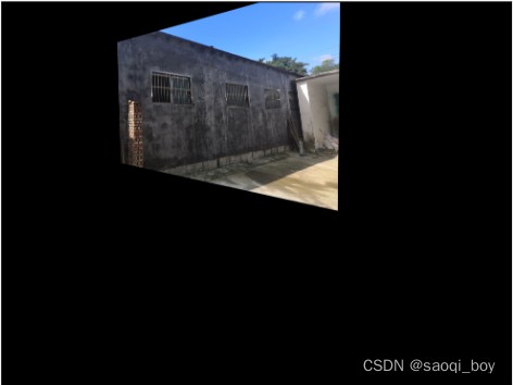
特征匹配圖:
圖像拼接結果: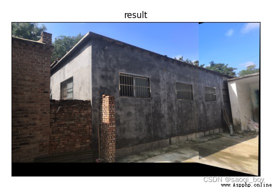
為圖片制作掩膜:
img = cv2.imread("img_1.png")
lower = np.uint8([120, 120, 120])
upper = np.uint8([255, 255, 255])
# [0,0,0] < lower < [255,255,255] < upper < [0,0,0]
mask = cv2.inRange(img, lower, upper)
showImage("mask", mask)
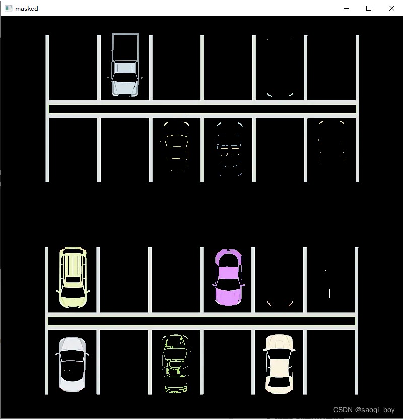
用mask提取圖片關鍵部分:
masked_img = cv2.bitwise_and(img, img, mask=mask)
showImage("masked", masked_img)
邊緣檢測:
gray_img = cv2.cvtColor(masked_img, cv2.COLOR_BGR2GRAY)
# 邊緣檢測
edge_img = cv2.Canny(gray_img, 50, 200)
showImage("edge", edge_img)
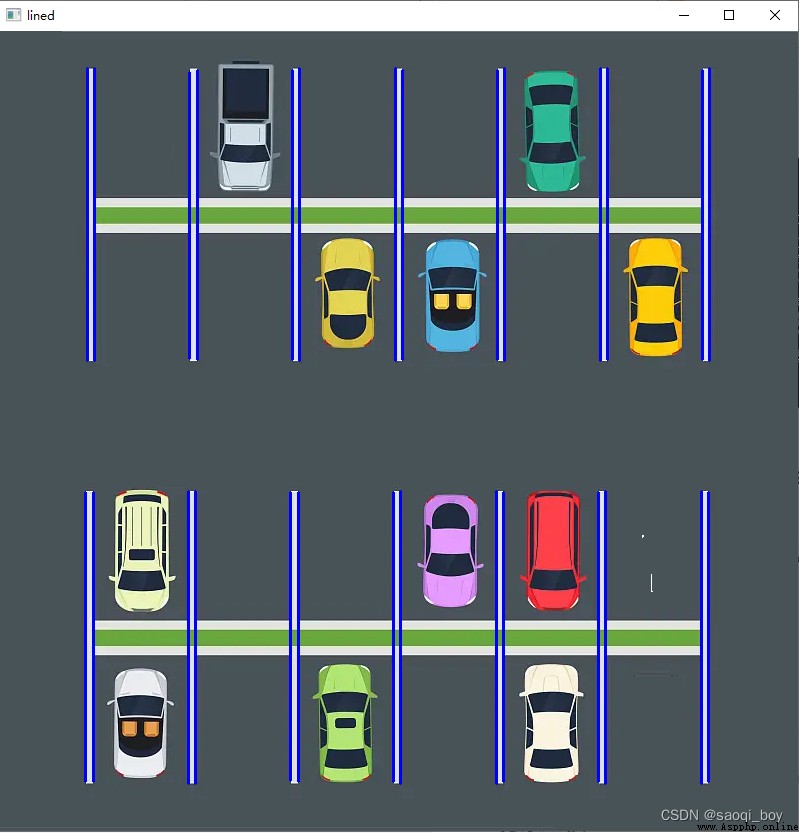
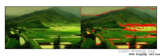
搜索邊緣中的直線並進行篩選:
# 直線檢測 rho:距離精度, theta:角度精度,threshold:阈值,minLineLength:最小線長,maxLineGap:最大間隔
lines = list(cv2.HoughLinesP(edge_img, rho=0.1, theta=np.pi/10, threshold=15, minLineLength=80, maxLineGap=50))
line_img = img.copy()
# 過濾
good = []
for line in lines:
for x1, y1, x2, y2 in line:
if abs(x2-x1) <= 1 and abs(y2-y1) >= 180:
good.append((x1, y1, x2, y2))
cv2.line(line_img, (x1, y1), (x2, y2), [255, 0, 0], thickness=2)
showImage("lined", line_img)
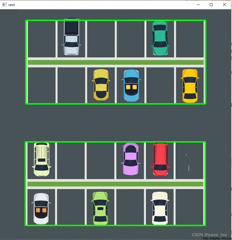
按行聚簇停車位:
import operator
# 按照y1排序
list1 = sorted(good, key=operator.itemgetter(1))
# 按行聚簇
clusters = {
}
dIndex = 0
clus_dist = 10
for i in range(len(list1) - 1):
distance = abs(list1[i+1][1] - list1[i][1])
if distance < clus_dist:
if not dIndex in clusters.keys():
clusters[dIndex] = []
clusters[dIndex].append(list1[i])
clusters[dIndex].append(list1[i+1])
else:
dIndex += 1
rects = {
}
i = 0
for key in clusters:
all_list = clusters[key]
cleaned = list(set(all_list))
if len(cleaned) > 3:
cleaned = sorted(cleaned, key=lambda tup: tup[0])
avg_x1 = cleaned[0][0]
avg_x2 = cleaned[-1][0]
avg_y1 = 0
avg_y2 = 0
for tup in cleaned:
avg_y1 += tup[1]
avg_y2 += tup[3]
avg_y1 = avg_y1/len(cleaned)
avg_y2 = avg_y2/len(cleaned)
rects[i] = (avg_x1, avg_y1, avg_x2, avg_y2)
i += 1
rects_img = img.copy()
for key in rects:
tup_topLeft = (int(rects[key][0]), int(rects[key][1]))
tup_botRight = (int(rects[key][2]), int(rects[key][3]))
cv2.rectangle(rects_img, tup_topLeft, tup_botRight, (0, 255, 0), 3)
showImage("rect", rects_img)
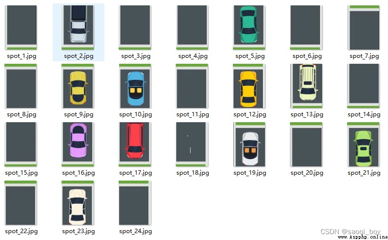
制作停車位標簽並保存每個停車位的圖片以用於後續模型訓練:
# 分割,制作標號字典
spot_dict = {
}
for key in rects:
x1, y1, x2, y2 = rects[key]
dis_x = abs(x2 - x1)/6
dis_y = abs(y1 - y2)/2
for i in range(6):
spot_dict[i+1+int(key)*6*2] = (int(x1 + i*dis_x), int(y2), int(x1 + (i+1)*dis_x), int(y2 + dis_y))
spot_dict[i+7+int(key)*6*2] = (int(x1 + i*dis_x), int(y2+dis_y), int(x1 + (i+1)*dis_x), int(y1))
# 寫入訓練圖片
import os
def writeImage():
cwd = os.getcwd()
for key in spot_dict:
(x1, y1, x2, y2) = spot_dict[key]
filename = "img/train/spot_" + str(key) + ".jpg"
spot_img = img[y1:y2, x1:x2]
cv2.imwrite(filename, spot_img)
writeImage()
這裡用的是pytorch框架訓練的模型,由於判斷0,1問題比較簡單,這裡僅展示模型結構
模型結構:
class MyModel(nn.Module):
def __init__(self):
super().__init__()
self.initial = nn.Sequential(
nn.Conv2d(3, 64, 3, 2, 1, padding_mode="reflect"),
nn.BatchNorm2d(64),
nn.ReLU()
)
self.body = nn.Sequential(
nn.Conv2d(64, 32, 3, 2, 1, padding_mode="reflect"),
nn.BatchNorm2d(32),
nn.ReLU(),
nn.Conv2d(32, 16, 3, 2, 1, padding_mode="reflect"),
nn.BatchNorm2d(16),
nn.ReLU(),
nn.Conv2d(16, 4, 3, 2, 1, padding_mode="reflect"),
nn.BatchNorm2d(4),
nn.ReLU(),
nn.AvgPool2d(4, 7)
)
self.fn = nn.Linear(4, 2)
def forward(self, x):
x = self.initial(x)
x = self.body(x)
x = torch.flatten(x, 1)
return self.fn(x)
更換圖片進行測試,圖片由同樣的方法進行車位分割,並由模型對每個位置進行判斷,處理代碼與上面相同,除了不再調用writeImage() :
# 更換圖片後,判斷
# 加載模型
from train import MyModel, DEVICE
from utils import load_checkpoint
from dataset import trans
import torch
def empty_detect():
empty = 0
result_img = img.copy()
model = MyModel().to(DEVICE)
load_checkpoint("spoting_judge.pth.tar", model)
model.eval()
with torch.no_grad():
for key in spot_dict:
(x1, y1, x2, y2) = spot_dict[key]
spot_img = img[y1:y2, x1:x2]
spot_img = cv2.cvtColor(spot_img, cv2.COLOR_BGR2RGB)
spot_img = trans(spot_img).unsqueeze(0).to(DEVICE)
output = model(spot_img)
_, not_empty = torch.max(output.data, 1) # 獲得最大值索引
if not not_empty:
empty += 1
cv2.rectangle(result_img, (x1, y1), (x2, y2), (0, 0, 255), 2)
cv2.putText(result_img, "empty:{}/{}".format(empty, len(spot_dict)), (10, 20), cv2.FONT_HERSHEY_SIMPLEX, 0.75, (0, 0, 255), 1, cv2.LINE_AA)
showImage("result", result_img)
empty_detect()
左上角顯示空車位個數,並將空車位用紅框標記顯示: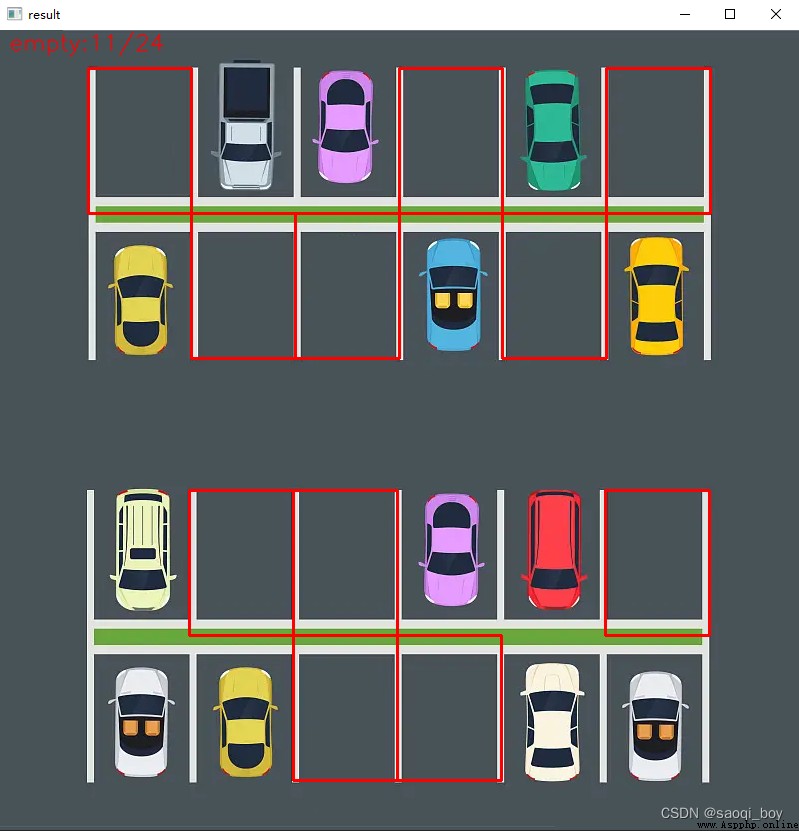
所謂背景建模就是通過計算前後幀的像素變化來分離出運動的物體,這裡用的方法是高斯混合模型:createBackgroundSubtractorMOG2()
import numpy as np
import cv2
cap = cv2.VideoCapture("video.mp4")
# 開運算需要的kernel:3*3的橢圓結構
kernel = cv2.getStructuringElement(cv2.MORPH_ELLIPSE, (3, 3))
# 創建混合高斯模型用於背景建模,參數介紹:
# history:用於訓練背景的幀數,默認幀數為500幀;
# varThreshold:方差阈值,用於判斷當前像素是前景還是背景,一般默認為16.如果光照變化明顯,如陽光下的水
# 面,建議設為25,值越大靈敏度越低;
# detectShadows:是否檢測影子,設為true為檢測,false為不檢測,一般設置為false;
fgbg = cv2.createBackgroundSubtractorMOG2()
while 1:
ret, frame = cap.read()
fgmask = fgbg.apply(frame)
# 開運算去噪點
fgmask = cv2.morphologyEx(fgmask, cv2.MORPH_OPEN, kernel)
# 尋找輪廓
contours, hierarchy = cv2.findContours(fgmask, cv2.RETR_EXTERNAL, cv2.CHAIN_APPROX_SIMPLE)
for c in contours:
# 計算周長
perimeter = cv2.arcLength(c, True)
if perimeter > 500:
x, y, w, h = cv2.boundingRect(c)
cv2.rectangle(frame, (x, y), (x+w, y+h), (0, 255, 0), 2)
cv2.imshow("dance", frame)
cv2.imshow("dance people", fgmask)
k = cv2.waitKey(100) & 0xff
if k == 27:
break
cap.release()
cv2.destroyAllWindows()
其中一幀: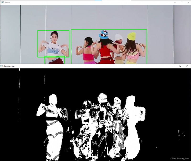
這裡主要用calcOpticalFlowPyrLK()進行光流估計,根據前後幀的特征點跟蹤特征點的位置。
參數介紹:
import numpy as np
import cv2
cap = cv2.VideoCapture("video.mp4")
feature_params = dict(
maxCorners=100,
qualityLevel=0.3,
minDistance=7
)
lk_params = dict(winSize=(15, 15), maxLevel=2)
color = np.random.randint(0, 255, (100, 3))
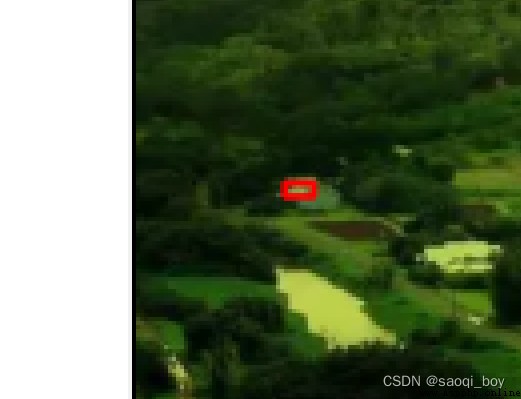
# 從570幀開始檢測
for _ in range(570):
cap.read()
ret, old_frame = cap.read()
old_gray = cv2.cvtColor(old_frame, cv2.COLOR_BGR2GRAY)
p0 = cv2.goodFeaturesToTrack(old_gray, mask=None, **feature_params)
mask = np.zeros_like(old_frame)
while True:
ret, frame = cap.read()
frame_gray = cv2.cvtColor(frame, cv2.COLOR_BGR2GRAY)
p1, st, err = cv2.calcOpticalFlowPyrLK(old_gray, frame_gray, p0, None, **lk_params)
good_new = p1[st == 1]
good_old = p0[st == 1]
for i, (new, old) in enumerate(zip(good_new, good_old)):
a, b = new.ravel()
c, d = old.ravel()
mask = cv2.line(mask, (int(a), int(b)), (int(c), int(d)), color[i].tolist(), 2)
frame = cv2.circle(frame, (int(a), int(b)), 5, color[i].tolist(), -1)
img = cv2.add(frame, mask)
# cv2.putText(img, "frame:{}th".format(j), (10, 20), cv2.FONT_HERSHEY_SIMPLEX, 0.75, (0, 0, 255), 1, cv2.LINE_AA)
cv2.imshow("frame", img)
if cv2.waitKey(100) & 0xff == 27:
break
old_gray = frame_gray.copy()
p0 = good_new.reshape(-1, 1, 2)
cap.release()
cv2.destroyAllWindows()
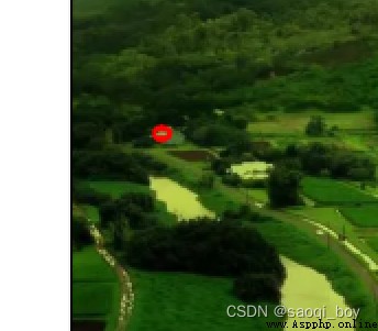
一些關鍵點的軌跡: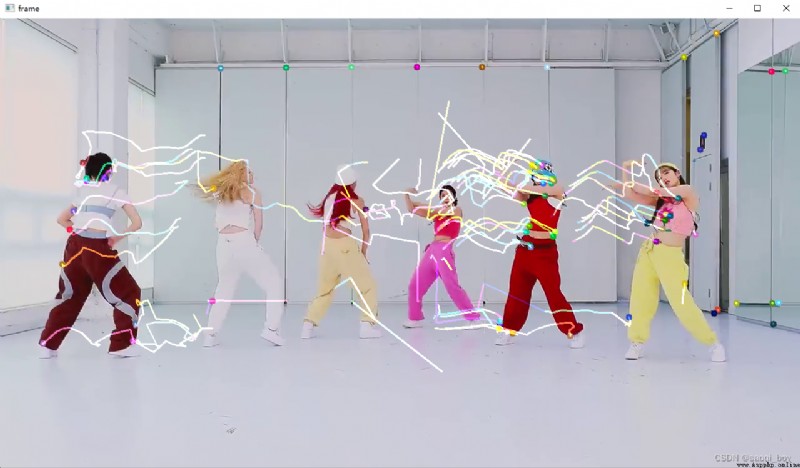
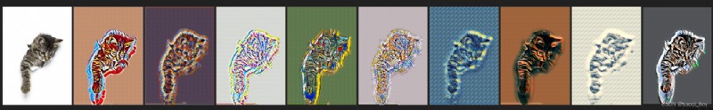
這裡以pytorch模型為例,加載的是風格遷移的模型,git地址:https://github.com/jcjohnson/fast-neural-style。blobFromImage()用於對圖像進行預處理,參數:
可選參數
import cv2
model_base_dir = "./models/total_model/"
# 為不同風格模型制作字典
modelName_map = {

1: "udnie",
2: "la_muse",
3: "the_scream",
4: "candy",
5: "mosaic",
6: "feathers",
7: "starry_night",
8: "composition_vii",
9: "the_wave"
}
def get_model_from_style(style: int):
""" 加載指定風格的模型 :param style: 模型編碼 :return: model """
model_name = modelName_map.get(style)
model_path = model_base_dir + model_name + ".t7"
model = cv2.dnn.readNetFromTorch(model_path)
return model
for i in range(len(modelName_map)):
net = get_model_from_style(i + 1)
img = cv2.imread("cat.jpg")
(h, w) = img.shape[:2]
blob = cv2.dnn.blobFromImage(img, 1.0, (w, h), (103.939, 116.779, 123.680), swapRB=False, crop=False)
net.setInput(blob)
output = net.forward()
output = output.reshape((3, output.shape[2], output.shape[3]))
output[0] += 103.939
output[1] += 116.779
output[2] += 123.680
output = output.transpose(1, 2, 0)
cv2.imwrite(modelName_map[i+1]+'.jpg', output)
各種風格的合影,最左邊為原圖,右邊風格依此按modelName_map排列 :
暫時懶得寫了,有空再更,找了個相似的:
https://blog.csdn.net/zxjoke/article/details/125657110
參考資料:
https://www.bilibili.com/video/BV1PV411774y
http://www.eepw.com.cn/article/202007/415158.htm