Python version CV - histogram 】 & Fourier transform

文章目錄

• • • 1、直方圖
    • • mask操作：
      • shape學習
      • 圖像基本運算：
      • 直方圖均衡化
    • 2、傅裡葉變換
    • • 傅裡葉變換的作用
      • 濾波：
      • 低通濾波器
      • 高通濾波器

1、直方圖

說明：統計像素值,Use a column chart for statistics

cv.calcHist(images,channels,mask,histSize,ranges)

• images：The format of the original image is uint8或者float32.當傳入函數時,Apply parentheses[]括起來,如：[image]
• channels：Also enclosed in parentheses,Tell the function that we unify the histogram of the image.如果入圖像是灰度圖它的值就是[0],如果是彩色圖,它的值可以是[0]、[1]、[2],對應B、G、R
• mask：掩膜圖像.Set it to unify the histogram of the entire imageNone,But if you want to unify the histogram of a certain part of the whole image make a mask image and use that.
• histSize： BIN的數目,括號括起來（一般固定256）
• ranges：像素范圍[0,256]（一般固定）

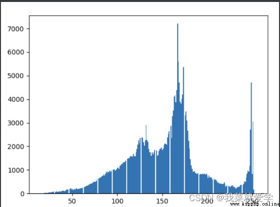
#直方圖
img=cv.imread("E:\\Pec\\cat.jpg",0)
hist=cv.calcHist([img],[0],None,[256],[0,256])
print(hist.shape)
plt.hist(img.ravel(),256)
plt.show()
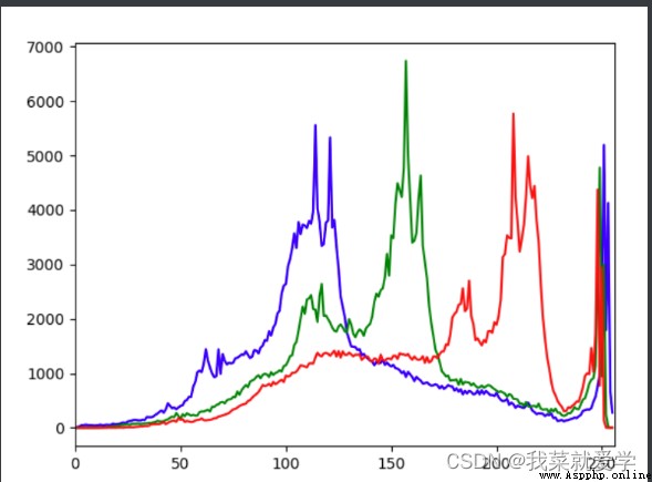
#彩色圖
img=cv.imread("E:\\Pec\\cat.jpg")
color=('b','g','r')
for i,col in enumerate(color):
histr=cv.calcHist([img],[i],None,[256],[0,256])
plt.plot(histr,color=col)
plt.xlim([0,256])
plt.show()

mask操作：

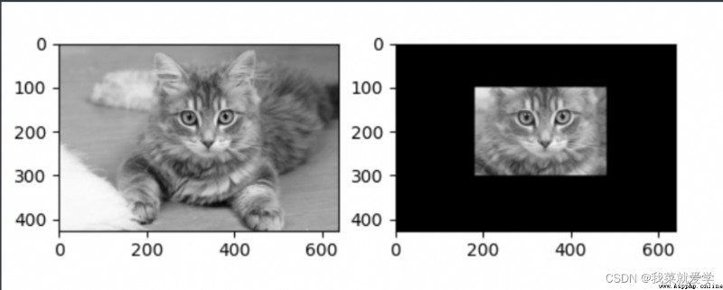
掩碼（mask）：只有兩部分,Part of it is black,The other part is white.

img=cv.imread("E:\\Pec\\cat.jpg",0)
mask_1=np.zeros(img.shape[:2],np.uint8)
print(mask_1.shape)
#Select some areas
mask_1[100:300,180:480]=255
#[100:300]Indicates up and down100位置到300,Go around in the same way180位置到480
cv_show('mask',mask_1)
masked_img=cv.bitwise_and(img,img,mask=mask_1)#與操作,maskIndicates the region to extract
cv_show('masked_img',masked_img)
plt.subplot(221),plt.imshow(img,'gray')
plt.subplot(222),plt.imshow(masked_img,'gray')
plt.show()
#plt.subplot(221) 表示將整個圖像窗口分為2行2列, 當前位置為1.
#plt.subplot(221) Represents the left image of the first row
#plt.subplot(222) 表示將整個圖像窗口分為2行2列, 當前位置為2.
#plt.subplot(222) 第一行的右圖
#plt.plot(line name）
#plt.xlim() 顯示的是xThe plot range of the axis
#plt.ylim() 顯示的是yThe plot range of the axis

shape學習

1. shape[:2] Take the length and width of the color picture
   shape[:3]Take the length and width and channel of the color picture
   

2. img.shape[0]:The vertical height of the image
   img.shape[1]:The horizontal width of the image
   img.shape[2]:圖像的通道數
   

3. 矩陣中,[0]代表水平,[1]代表高度.
   

   print(type(img)) #顯示類型
   print(img.shape) #顯示尺寸
   print(img.shape[0]) #圖片寬度
   print(img.shape[1]) #圖片高度
   print(img.shape[2]) #圖片通道數
   print(img.size) #顯示總像素個數
   print(img.max()) #最大像素值
   print(img.min()) #最小像素值
   print(img.mean()) #像素平均值
   print(img.shape[:0])
   print(img.shape[:1])#圖片寬度
   print(img.shape[:2])#圖片寬度,高度
   print(img.shape[:3])#圖片寬度,高度,通道數
   

圖像基本運算：

說明：圖像的基本運算有很多種,比如兩幅圖像可以相加、相減、相乘、相除、位運算、平方根、對數、絕對值等;圖像也可以放大、縮小、旋轉,還可以截取其中的一部分作為ROI（感興趣區域）進行操作,各個顏色通道還可以分別提取及對各個顏色通道進行各種運算操作.

#bitwise_and、bitwise_or、bitwise_xor、bitwise_not這四個按位操作函數.
void bitwise_and(InputArray src1, InputArray src2,OutputArray dst, InputArray mask=noArray()); //dst = src1 & src2
void bitwise_or(InputArray src1, InputArray src2,OutputArray dst, InputArray mask=noArray()); //dst = src1 | src2
void bitwise_xor(InputArray src1, InputArray src2,OutputArray dst, InputArray mask=noArray()); //dst = src1 ^ src2
void bitwise_not(InputArray src, OutputArray dst,InputArray mask=noArray()); //dst = ~src

• bitwise_and是對二進制數據進行“與”操作,即對圖像（灰度圖像或彩色圖像均可）每個像素值進行二進制“與”操作,1&1=1,1&0=0,0&1=0,0&0=0
• bitwise_or是對二進制數據進行“或”操作,即對圖像（灰度圖像或彩色圖像均可）每個像素值進行二進制“或”操作,1|1=1,1|0=0,0|1=0,0|0=0
• bitwise_xor是對二進制數據進行“異或”操作,即對圖像（灰度圖像或彩色圖像均可）每個像素值進行二進制“異或”操作,1^1=0,10=1,0^1=1,00=0
• bitwise_not是對二進制數據進行“非”操作,即對圖像（灰度圖像或彩色圖像均可）每個像素值進行二進制“非”操作,_1=0,0=1

直方圖均衡化

img=cv.imread("E:\\Pec\\cat.jpg",0)
hist=cv.calcHist([img],[0],None,[256],[0,256])
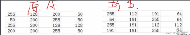
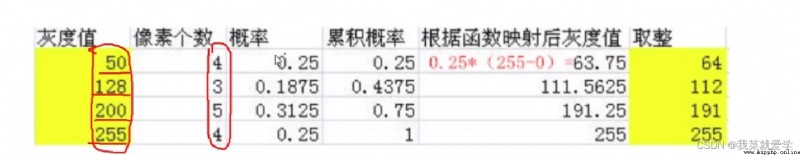
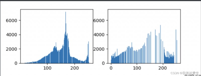
#均衡化
equ=cv.equalizeHist(img)
plt.subplot(221),plt.hist(img.ravel(),256)
plt.subplot(222),plt.hist(equ.ravel(),256)
plt.show()
res=np.hstack((img,equ))
cv_show("red",res)

2、傅裡葉變換

說明：Live in the world of time,早上7:00吃早飯,8:00上班路上,9:00上班,Time-referenced time domain analysis.In the frequency domain everything appears to be stationary,以上帝的視角.There is no need to know when and what you did in order,Just need to know what you did during the day

傅裡葉變換的作用

• 高頻：The transformation is violent to obtain the grayscale components,例如邊界
• 低頻：變化緩慢的灰度分量,For example, the endless sea

濾波：

• 低通濾波器：只保留低頻,會使圖像變得模糊
• 高通濾波器：只保留高頻,Enhances image detail

注意：

（1）輸入圖像需要先轉換成np.float32格式

（2）The result obtained in the frequency domain is 0的部分會在左上角,Usually to go to the center,可以通過shift變換來實現

（3）cv.dft()返回的結果是雙通道的(實部,虛部),Usually need to convert to image format to display（0,255）

補充：

（1）numpy.zeros(shape, dtype=float)

• 各個參數意義：
  shape：創建的新數組的形狀（維度）.
  dtype：創建新數組的數據類型.
• 返回值：給定維度的全零數組.

（2）numpy.ones(shape, dtype=None, order=‘C’)

• 可以創建任意維度和元素個數的數組,其元素值均為1
• shape ：int或int的序列,為新數組的形狀;
• dtype（可選 ）：數組的所需數據類型;默認是 numpy.float64.
• order ： {‘C’,‘F’},可選,默認值：C 是否在內存中以行主（C-風格）或列主（Fortran-風格）順序存儲多維數據.

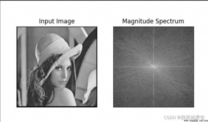
img=cv.imread("E:\\Pec\\lida.jpg",0)
img_float32=np.float32(img)#輸入圖像需要先轉換成np.float32格式
#Fourier transform to complex numbers
dft=cv.dft(img_float32,flags=cv.DFT_COMPLEX_OUTPUT)
#Translate low frequencies from top left to center
dft_shift=np.fft.fftshift(dft)
#得到灰度圖能表示的形式
#cv.dft()返回的結果是雙通道的(實部,虛部),Usually need to convert to image format to display（0,255）
magnitude_spectrum=20*np.log(cv.magnitude(dft_shift[:,:,0],dft_shift[:,:,1]))
plt.subplot(121),plt.imshow(img,'gray')
plt.title('Input Image'),plt.xticks([]),plt.yticks([])
plt.subplot(122),plt.imshow(magnitude_spectrum,'gray')
plt.title('Magnitude Spectrum'),plt.xticks([]),plt.yticks([])
plt.show()

低通濾波器

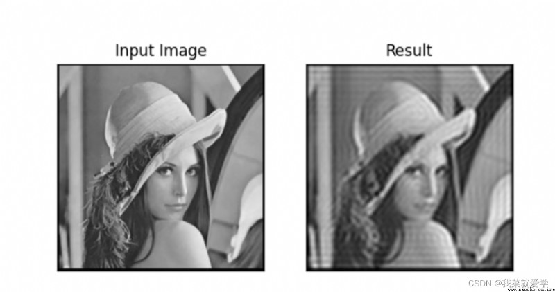
#低通濾波器
img=cv.imread("E:\\Pec\\lida.jpg",0)
img_float32=np.float32(img)#輸入圖像需要先轉換成np.float32格式
#Fourier transform to complex numbers
dft=cv.dft(img_float32,flags=cv.DFT_COMPLEX_OUTPUT)
#Translate low frequencies from top left to center
dft_shift=np.fft.fftshift(dft)
#Find the image center position
rows,cols=img.shape
crow,col=int(rows/2),int(cols/2)
#低通濾波
#生成rows行cols列的2緯矩陣,數據格式為uint8,uint8的范圍[0,255]
mask=np.zeros((rows,cols,2),np.uint8)
mask[crow-30:crow+30,col-30:col+30]=1
#IDFT
fshift=dft_shift*mask
f_ishift=np.fft.ifftshift(fshift)
img_back=cv.idft(f_ishift)
img_back=cv.magnitude(img_back[:,:,0],img_back[:,:,1])
plt.subplot(121),plt.imshow(img,'gray')
plt.title('Input Image'),plt.xticks([]),plt.yticks([])
plt.subplot(122),plt.imshow(img_back,'gray')
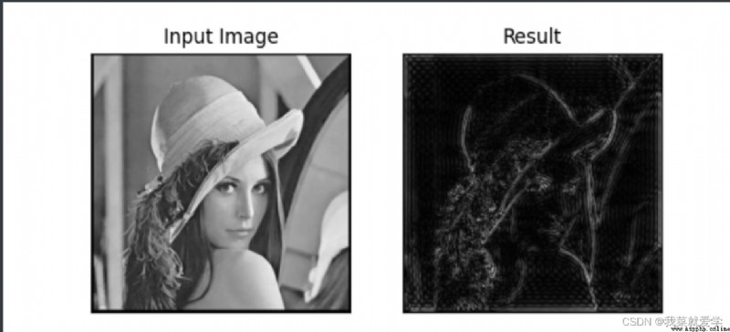
plt.title('Result'),plt.xticks([]),plt.yticks([])
plt.show()

從結果可以看出,The edges of the image are blurred,But the image is not blurry except for the edge parts

高通濾波器

#高通濾波
#生成rows行cols列的2緯矩陣,數據格式為uint8,uint8的范圍[0,255]
mask=np.ones((rows,cols,2),np.uint8)
mask[crow-30:crow+30,col-30:col+30]=0

從結果可以看出,Only the edge information of the image is preserved,The content is blurred and gone