At the beginning : After learning the basic operation of image in the previous article , This blog is a part of recording image processing . review python Version of OpenCV Second articles , I also have a certain understanding of related image processing . Video reference B standing Dr. Tang Yudi , It is also recommended by a computer vision boss .
ret,dst=cv2.threshold(src,thresh,maxval,type)
src: Input diagram , Only single channel images can be input , It is generally a grayscale image
dst: Output chart
thresh: threshold
maxval: When the pixel value exceeds the threshold ( Or less than the threshold ), The value assigned to
type: Two valued ( Greater than take a value , Less than take another value ) Type of operation , There are five types of
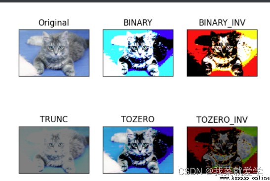
THRESH_BINARY: The part exceeding the threshold is taken as maxval, Otherwise 0
THRESH_BINARY_INV: THRESH_BINARY The reversal of
THRESH_TRUNC: The part greater than the threshold is set as the threshold , Otherwise unchanged
THRESH_TOZERO: Parts larger than the threshold do not change , Otherwise, it is set to 0
THRESH_TOZERO_INV: THRESH_TOZERO The reversal of
# Image threshold
# Show the original
#img=cv.cvtColor(img,cv.COLOR_BGR2GRAY) # Image graying
cv_show("yuantu",img)
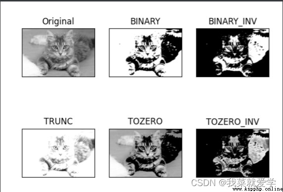
ret,thresh1=cv.threshold(img,127,255,cv.THRESH_BINARY)
ret,thresh2=cv.threshold(img,127,255,cv.THRESH_BINARY_INV)
ret,thresh3=cv.threshold(img,127,255,cv.THRESH_TRUNC)
ret,thresh4=cv.threshold(img,127,255,cv.THRESH_TOZERO)
ret,thresh5=cv.threshold(img,127,255,cv.THRESH_TOZERO_INV)
title=['Original','BINARY','BINARY_INV','TRUNC','TOZERO','TOZERO_INV']
images=[img,thresh1,thresh2,thresh3,thresh4,thresh5]
for i in range(6):
plt.subplot(2,3,i+1),plt.imshow(images[i],'gray')
plt.title(title[i])
plt.xticks([]),plt.yticks([])
plt.show()
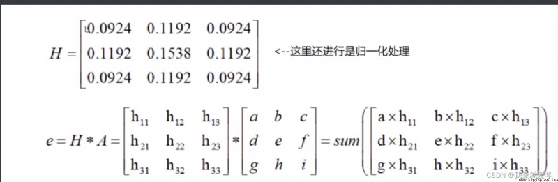
explain : By constructing a convolution matrix , Do inner product .
image=cv.imread('E:\\Pec\\zao.jpg')
cv.imshow('image',image)
cv.waitKey(0)
cv.destroyAllWindows() # If you haven't released memory before destroyallWIndows Will release the memory occupied by that variable
# Simple average convolution operation
blur=cv.blur(image,(3,3))
#cv_show('blur',blur)
explain : Basically the same as mean filtering , You can choose to normalize
box=cv.boxFilter(image,-1,(3,3),normalize=False)#-1 Indicates that the input elements are consistent .
# normalize=True It means normalization , And mean filtering has been . if false, Don't do it , Do not divide by the length and width of the matrix , But it's easy to cross the border .
# Greater than 255, Then take 255
#cv_show('box',box)

explain : The value in the convolution kernel of Gaussian blur satisfies the Gaussian distribution ( It's a convex curve , Pay more attention to the middle )
aussian=cv.GaussianBlur(image,(5,5),1)
#cv_show('aussian',aussian)
explain : Take a convolution , Then take the intermediate value instead
median=cv.medianBlur(image,5)
#cv_show("median",median)
# Focus on
res=np.hstack((blur,aussian,median))
#np.hatack: Stack arrays horizontally , Form a new array
#np.vstack: Stack arrays vertically , Form a new array
print(res)
cv_show("average",res)
[[[226 134 53]
[226 134 53]
[226 134 53]
...
[226 134 53]
[226 134 53]
[226 134 53]]

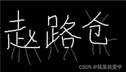
# morphology - Corrosion operation
image=cv.imread('E:\\Pec\\fushi.jpg')
cv_show("fushi-Ori",image)
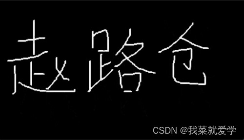
kernel=np.ones((2,2),np.uint8)#(2,2) Indicates the size of the corroded core , Is the radius of corrosion
erosion=cv.erode(image,kernel,iterations=1)#iterations=1 Indicates the number of corrosion
cv_show("fushi-eff",erosion)
Original picture :
After corrosion :
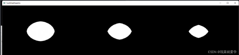
Then continuous pictures introduce the corrosion process :
pie=cv.imread('E:\\Pec\\fushiyuan.jpg')
cv_show("pie",pie)
kernel=np.ones((20,20),np.uint8)
erosion1=cv.erode(pie,kernel,iterations=1)
erosion2=cv.erode(pie,kernel,iterations=2)
erosion3=cv.erode(pie,kernel,iterations=3)
res=np.hstack((erosion1,erosion2,erosion3))
cv_show('fushilianhuantu',res)

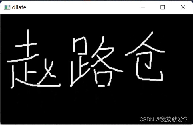
# morphology - Expansion operation
image=cv.imread('E:\\Pec\\fushi.jpg')
cv_show("fushi-Ori",image)
kernel=np.ones((3,3),np.uint8)#(2,2) Indicates the size of the corroded core , Is the radius of corrosion
erosion=cv.erode(image,kernel,iterations=1)#iterations=1 Indicates the number of corrosion
cv_show("fushi-eff",erosion)
dige_dilate=cv.dilate(erosion,kernel,iterations=1)
cv_show('dilate',dige_dilate)
# open : Corrode first , Re expansion
image=cv.imread('E:\\Pec\\fushi.jpg')
kernel=np.ones((3,3),np.uint8)#(2,2) Indicates the size of the corroded core , Is the radius of corrosion
opening=cv.morphologyEx(image,cv.MORPH_OPEN,kernel)
#cv_show("opening",opening)
# close : Inflate first , Corrode again
image=cv.imread('E:\\Pec\\fushi.jpg')
kernel=np.ones((3,3),np.uint8)#(2,2) Indicates the size of the corroded core , Is the radius of corrosion
closeing=cv.morphologyEx(image,cv.MORPH_CLOSE,kernel)
#cv_show("close",closeing)
res=np.hstack((image,opening,closeing))
cv_show('fushilianhuantu',res)
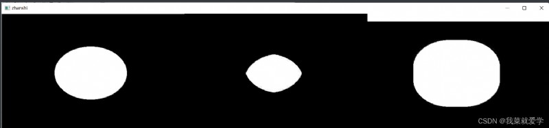
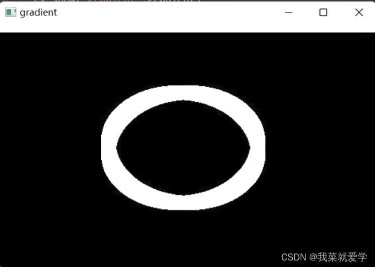
explain :# gradient = inflation - corrosion
pie=cv.imread('E:\\Pec\\fushiyuan.jpg')
kernel=np.ones((20,20),np.uint8)
erode=cv.erode(pie,kernel,iterations=2)
dilate=cv.dilate(pie,kernel,iterations=2)
res=np.hstack((pie,erode,dilate))
cv_show("zhanshi",res)
gradient=cv.morphologyEx(pie,cv.MORPH_GRADIENT,kernel)
cv_show("gradient",gradient)
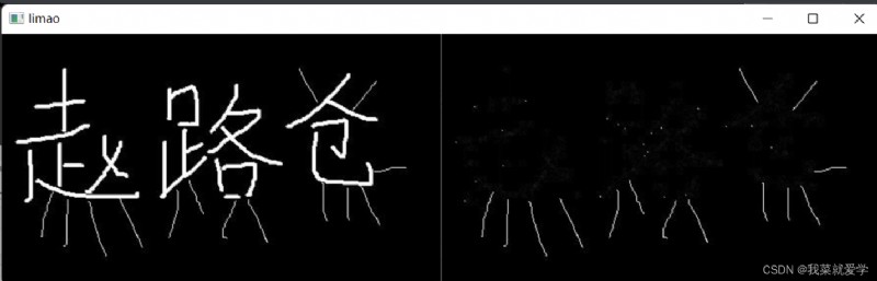
# Top hat and black hat
image=cv.imread('E:\\Pec\\fushi.jpg')
kernel=np.ones((3,3),np.uint8)#(2,2) Indicates the size of the corroded core , Is the radius of corrosion
topat=cv.morphologyEx(image,cv.MORPH_TOPHAT,kernel)
res=np.hstack((image,topat))
cv_show("limao",res)
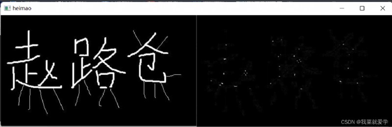
blackhat=cv.morphologyEx(image,cv.MORPH_BLACKHAT,kernel)
res=np.hstack((image,blackhat))
cv_show("heimao",res)
explain :
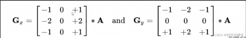
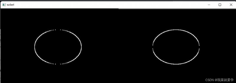
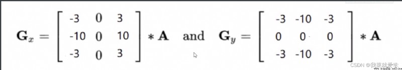
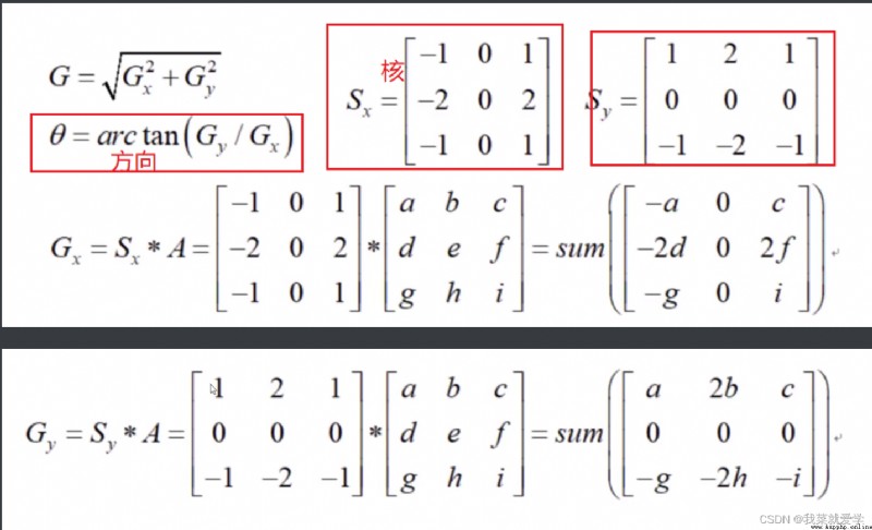
Sobel Operator is one of the most important operators in pixel image edge detection . On the technical , It is a discrete first-order difference operator , Used to calculate the approximate value of one step of image brightness function . Use this operator at any point in the image , The gradient vector or its normal vector corresponding to the point will be generated . This method can highlight the contour features of the image by enhancing the edge effect of the image .
Why detect edges ?
For example, in autopilot , At least one of our jobs is road edge detection , Only by correctly detecting the edge of the road, our car will drive on the road instead of driving out of the road .
Or explain it from another angle , We do edge detection not to let the human eye appreciate the road edge in a road picture , We correctly detect the edge of an image in order to make the model better understand the road in this image . Therefore, accurate edge detection can help computer models identify whether it is a road or outside the road , So as to make correct feedback —— Guide the car to operate correctly .
d s t = c v . S o b e l ( s r c , d d e p t h , d x , d y , k s i z e ) dst=cv.Sobel(src,ddepth,dx,dy,ksize) dst=cv.Sobel(src,ddepth,dx,dy,ksize)
#cv.CV_64F,opencv By default, the negative value is redefined as 0. Add this to allow negative values
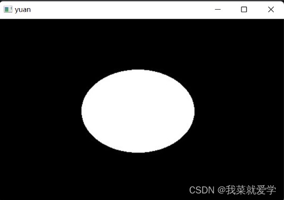
pie=cv.imread('E:\\Pec\\fushiyuan.jpg')
cv_show("yuan",pie)
sobelx=cv.Sobel(pie,cv.CV_64F,1,0,ksize=3)#1,0 Only the horizontal direction
# On the right - On the left : White to black is a positive number , Black to white is a negative number , All negative numbers will be truncated to 0, So take the absolute value
sobelx=cv.convertScaleAbs(sobelx)
#cv_show("sobelx",sobelx)
# In the vertical direction
sobely=cv.Sobel(pie,cv.CV_64F,0,1,ksize=3)#1,0 Only the horizontal direction
# On the right - On the left : White to black is a positive number , Black to white is a negative number , All negative numbers will be truncated to 0, So take the absolute value
sobely=cv.convertScaleAbs(sobely)
res=np.hstack((sobelx,sobely))
cv_show("sobel",res)
# If required Gx and Gy It is not recommended to add directly , Put the above (1,0) perhaps (0,1) It's written in (1,1)
sobelxy=cv.addWeighted(sobelx,0.5,sobely,0.5,0)# Is a saturation operation , By adding their respective weights
cv_show("sobelxy",sobelxy)

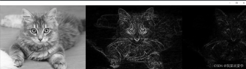
Specific examples :
# An example
pie=cv.imread('E:\\Pec\\cat.jpg')
ima=cv.cvtColor(pie,cv.COLOR_BGR2GRAY)
#cv_show("pie",ima)
sobelx=cv.Sobel(ima,cv.CV_64F,1,0,ksize=3)
sobelx=cv.convertScaleAbs(sobelx)
sobely=cv.Sobel(ima,cv.CV_64F,0,1,ksize=3)#1,0 Only the horizontal direction
sobely=cv.convertScaleAbs(sobely)
sobelxy=cv.addWeighted(sobelx,0.5,sobely,0.5,0)
#cv_show("sobelxy",sobelxy)
sobelxy1=cv.Sobel(ima,cv.CV_64F,1,1,ksize=3)#1,0 Only the horizontal direction
sobelxy1=cv.convertScaleAbs(sobelxy1)
#cv_show("sobelxy1",sobelxy1)
res=np.hstack((ima,sobelxy,sobelxy1))
cv_show("zong",res)
Make the value of convolution larger 、 More sensitive ; The description is more detailed
The second derivative , The rate of change of the first derivative ; More sensitive ; Sensitive to noise points ; Use with other operators

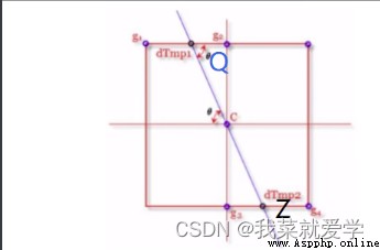
Linear interpolation : set up g1 The magnitude of the gradient M(g1),g2 The magnitude of the gradient M(g2), be dtmp1 You can get :
M ( d t m p 1 ) = w ∗ M ( g 2 ) + ( 1 − w ) ∗ M ( g 1 ) M(dtmp1)=w*M(g2)+(1-w)*M(g1) M(dtmp1)=w∗M(g2)+(1−w)∗M(g1)
w = d i s t a n c e ( d t m p 1 , g 2 ) / d i s t a n c e ( g 1 , g 2 ) / / d i s t a n c e ( g 1 , g 2 ) It means the distance between two points w=distance(dtmp1,g2)/distance(g1,g2) //distance(g1,g2) It means the distance between two points w=distance(dtmp1,g2)/distance(g1,g2)//distance(g1,g2) It means the distance between two points
Last , By calculation , Compare C Whether the point gradient amplitude is greater than Q、Z, Then suppress non maximum points

explain :minVal:80; MaxVal:150; Make it your own . if minVal When the setting is too small , The filtering range becomes smaller , The requirements are very low .maxVal Empathy
# edge detection
cat=cv.imread('E:\\Pec\\loufang.jpg',cv.IMREAD_GRAYSCALE)
v1=cv.Canny(cat,120,250)
#minVal:80; MaxVal:150; Make it your own .
# if minVal When the setting is too small , The filtering range becomes smaller , The requirements are very low .maxVal Empathy
v2=cv.Canny(cat,50,100)
res=np.hstack((v1,v2))
cv_show("res",res)
The results can be analyzed : The wider the range of threshold setting , The clearer the details of the image are described 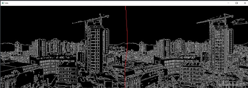
 100 days of proficiency in python (crawler) - day 44: summary of requests Library
List of articles Each preface
 Introduction to Python zero Basics - 08 - variables and keywords in Python
List of articles Python Variab