Catalog
Preface
brick : Neuron
A simple example
Encode a neuron
Assemble neurons into a network
Example : feedforward
Coding neural network : feedforward
Training neural network The first part
Loss
Examples of loss calculation
Code :MSE Loss
Training neural network The second part
Example : Calculating partial derivatives
Code : A complete neural network
The latter
We use Python Implement a... From scratch neural network To understand the principle of Neural Networks .
First, let's look at the basic units of Neural Networks , Neuron . Neurons accept input , Do some data operations on it , And then produce output . for example , This is a 2- Input neuron :
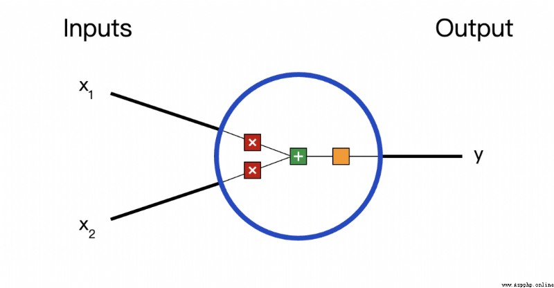
Three things happened here . First , Each input is multiplied by a weight ( Red ):

then , Weighted input summation , Add a deviation b( green ):

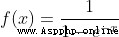
Last , This result is passed to an activation function f:

The purpose of the activation function is to put an unbounded input , Transform into a predictable form . The commonly used activation function is S Type of function :
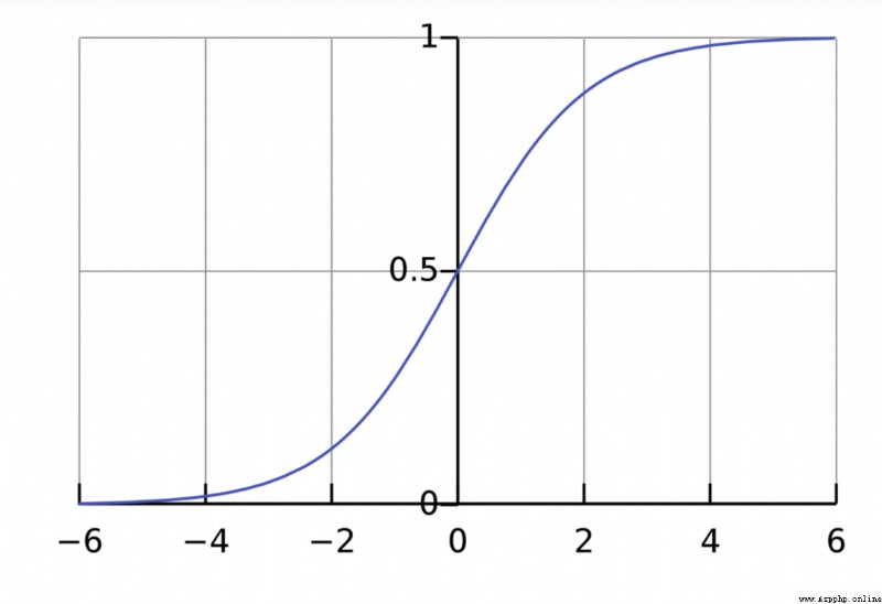
S The range of value of a type function is (0, 1). Simply speaking , Is to put (−∞, +∞) Compress to (0, 1) , A large negative number is about 0, A large positive number is about 1.
Suppose we have a neuron , The activation function is S Type of function , Its parameters are as follows :
w=[0,1],b=4
w=[0,1] It is expressed in the form of vectors w1=0,w2=1. Now? , We give this neuron an input [2,3]. We use dot product to express :

When the input is [2, 3] when , The output of this neuron is 0.999. A given input , The process of getting the output is called feedforward (feedforward).
Let's implement a neuron ! use Python Of NumPy Library to complete the mathematical calculation :
import numpy as np
def sigmoid(x):
# Our activation function : f(x) = 1 / (1 + e^(-x))
return 1 / (1 + np.exp(-x))
class Neuron:
def __init__(self, weights, bias):
self.weights = weights
self.bias = bias
def feedforward(self, inputs):
# Weighted input , Add bias , Then use the activation function
total = np.dot(self.weights, inputs) + self.bias
return sigmoid(total)
weights = np.array([0, 1]) # w1 = 0, w2 = 1
bias = 4 # b = 4
n = Neuron(weights, bias)
x = np.array([2, 3]) # x1 = 2, x2 = 3
print(n.feedforward(x)) # 0.9990889488055994
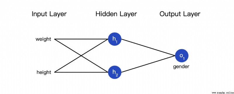
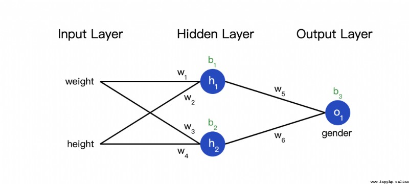
The so-called neural network is a pile of neurons . This is a simple neural network :
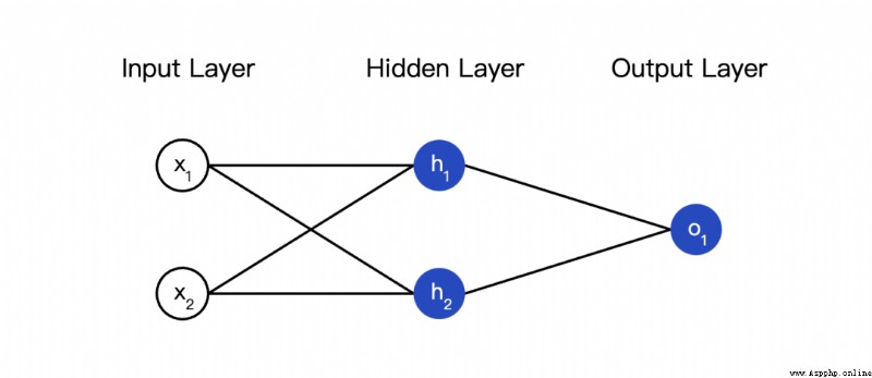
This network has two inputs , One has two neurons (  and
and  ) The hidden layer of , And one has a neuron (
 ) ) The output layer of . it is to be noted that , The input is and Output , This forms a network .
The hidden layer is the layer between the input layer and the output layer , Hidden layers can be multi-layered .
We continue to use the network in the previous figure , Suppose the weight of each neuron is , The intercept term is the same , Activation functions are also S Type of function . Use them separately Represents the output of the corresponding neuron .
When the input x=[2,3] when , What's going to happen ?
This neural network pairs inputs [2,3] The output of is 0.7216, It's simple .
import numpy as np
# ... code from previous section here
class OurNeuralNetwork:
''' A neural network with: - 2 inputs - a hidden layer with 2 neurons (h1, h2) - an output layer with 1 neuron (o1) Each neuron has the same weights and bias: - w = [0, 1] - b = 0 '''
def __init__(self):
weights = np.array([0, 1])
bias = 0
# Here are neurons from the previous section
self.h1 = Neuron(weights, bias)
self.h2 = Neuron(weights, bias)
self.o1 = Neuron(weights, bias)
def feedforward(self, x):
out_h1 = self.h1.feedforward(x)
out_h2 = self.h2.feedforward(x)
# o1 The input is h1 and h2 Output
out_o1 = self.o1.feedforward(np.array([out_h1, out_h2]))
return out_o1
network = OurNeuralNetwork()
x = np.array([2, 3])
print(network.feedforward(x)) # 0.7216325609518421
Results the correct , It doesn't look like a problem .
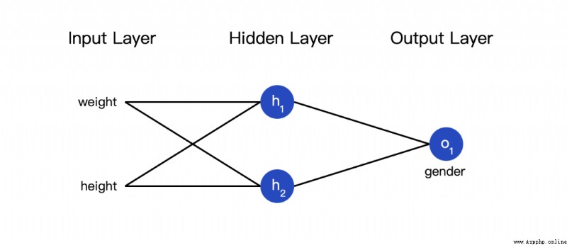
Now there are such data :
Next, we use this data to train the weight and intercept terms of the neural network , Thus, gender can be predicted according to height and weight :
We use it 0 and 1 It means male (M) And women (F), And the numerical value is transformed :
I chose it at random 135 and 66 To standardize data , The average value is usually used .
Before training the web , We need to quantify that the current network is 『 good 』 still 『 bad 』, So we can find a better network . This is the purpose of defining loss .
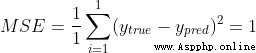
We use mean variance here (MSE) Loss : , Let's take a closer look :
n Is the number of samples , This is equal to 4(Alice、Bob、Charlie and Diana).
y Represents the variable to be predicted , Here is gender .
 Is the true value of the variable (『 right key 』). for example ,Alice Of Namely 1( men ).
 The predicted value of the variable . This is the output of our network .
 It is called variance (squared error). Our loss function is the average of all variances . Prediction effect Yu Hao , The less you lose .
Better prediction = Less loss !
Training network = Minimize its loss .
Suppose our network always outputs 0, In other words, think that everyone is male . How about the loss ?
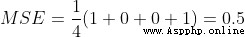
Here is the calculation MSE Lost code :
import numpy as np
def mse_loss(y_true, y_pred):
# y_true and y_pred are numpy arrays of the same length.
return ((y_true - y_pred) ** 2).mean()
y_true = np.array([1, 0, 0, 1])
y_pred = np.array([0, 0, 0, 0])
print(mse_loss(y_true, y_pred)) # 0.5
If you don't understand this code , You can see NumPy Quick start on Array Operations .
Now we have a clear goal : Minimize the loss of Neural Networks . By adjusting the weight and intercept of the network , We can change the prediction results , But how can we gradually reduce losses ?
This paragraph involves multivariate calculus , If you are not familiar with calculus , You can skip these mathematical contents .
This paragraph involves multivariate calculus , If you are not familiar with calculus , You can skip these mathematical contents .
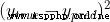
To simplify the problem , Suppose there are only Alice, Then the mean square loss is just Alice The variance of :
Loss can also be regarded as a function of weight and intercept terms . Let's label the network with the terms of weight and intercept :
In this way, we can express the loss of the network as :

Suppose we want to optimize  , When we change when , Loss
  How will it change ? It can be used
  To answer this question , How to calculate ?
First , Let's use it  To rewrite this Partial derivative :

Because we already know  , So we can calculate

Now let's take care of it . Are the outputs of the neurons they represent , We have :

because Will only affect ( Does not affect the ), therefore :

Yes  , We can do the same :


ad locum , It's height ,
 It's weight . This is the second time we've seen
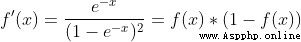
  (S The derivative of a type function ) 了 . solve :
We have It breaks down into several parts that we can calculate :

This method of calculating partial derivatives is called 『 Back propagation algorithm 』(backpropagation).
Many mathematical symbols , If you haven't figured it out , Let's look at a practical example .
Let's look at the data set, only Alice The situation of :
Initialize all weight and intercept terms to 1 and 0. Do feedforward calculation in the network :


The output of the network is  , about Male(0) perhaps Female(1) Not too inclined . Calculate it


Tips : The front has been S Derivative of activation function of type
.
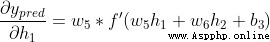
Get it done ! This result means to increase , It will also rise slightly .
Now everything is ready to train neural networks ! We will use an optimization algorithm called random gradient descent method to optimize the weight and intercept terms of the network , Minimize losses . The core is this update formula :

 It's a constant , It's called the learning rate , Used to adjust the speed of training . All we have to do is use subtract
Our training process is like this :
Select a sample from our data set , Optimize with random gradient descent method —— Each time we optimize only one sample ;
Calculate the partial derivative of each weight or intercept term to the loss ( for example 、 etc. );
Update each weight and intercept term with the update equation ;
Repeat the first step ;
We can finally realize a complete neural network :
Overall code
import numpy as np
def sigmoid(x):
# Sigmoid activation function: f(x) = 1 / (1 + e^(-x))
return 1 / (1 + np.exp(-x))
def deriv_sigmoid(x):
# Derivative of sigmoid: f'(x) = f(x) * (1 - f(x))
fx = sigmoid(x)
return fx * (1 - fx)
def mse_loss(y_true, y_pred):
# y_true and y_pred It's the same length numpy Array .
return ((y_true - y_pred) ** 2).mean()
class OurNeuralNetwork:
''' A neural network with: - 2 inputs - a hidden layer with 2 neurons (h1, h2) - an output layer with 1 neuron (o1) *** disclaimer ***: The following code is for simplicity and demonstration , Not the best . The real neural network code is completely different . Do not use this code . contrary , read / Run it to understand how this particular network works . '''
def __init__(self):
# The weight ,Weights
self.w1 = np.random.normal()
self.w2 = np.random.normal()
self.w3 = np.random.normal()
self.w4 = np.random.normal()
self.w5 = np.random.normal()
self.w6 = np.random.normal()
# Intercept item ,Biases
self.b1 = np.random.normal()
self.b2 = np.random.normal()
self.b3 = np.random.normal()
def feedforward(self, x):
# X Is a 2 A numeric array of elements .
h1 = sigmoid(self.w1 * x[0] + self.w2 * x[1] + self.b1)
h2 = sigmoid(self.w3 * x[0] + self.w4 * x[1] + self.b2)
o1 = sigmoid(self.w5 * h1 + self.w6 * h2 + self.b3)
return o1
def train(self, data, all_y_trues):
''' - data is a (n x 2) numpy array, n = # of samples in the dataset. - all_y_trues is a numpy array with n elements. Elements in all_y_trues correspond to those in data. '''
learn_rate = 0.1
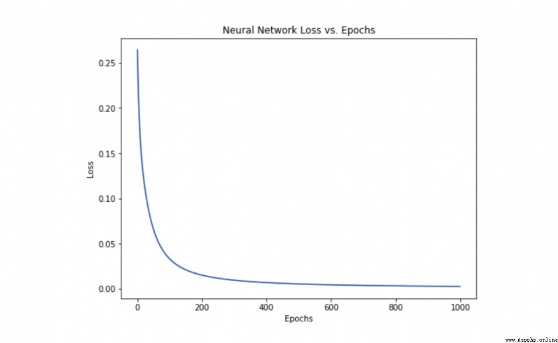
epochs = 1000 # Number of times to traverse the entire data set
for epoch in range(epochs):
for x, y_true in zip(data, all_y_trues):
# --- Make a feedforward ( We will need these values later )
sum_h1 = self.w1 * x[0] + self.w2 * x[1] + self.b1
h1 = sigmoid(sum_h1)
sum_h2 = self.w3 * x[0] + self.w4 * x[1] + self.b2
h2 = sigmoid(sum_h2)
sum_o1 = self.w5 * h1 + self.w6 * h2 + self.b3
o1 = sigmoid(sum_o1)
y_pred = o1
# --- Calculating partial derivatives .
# --- Naming: d_L_d_w1 represents "partial L / partial w1"
d_L_d_ypred = -2 * (y_true - y_pred)
# Neuron o1
d_ypred_d_w5 = h1 * deriv_sigmoid(sum_o1)
d_ypred_d_w6 = h2 * deriv_sigmoid(sum_o1)
d_ypred_d_b3 = deriv_sigmoid(sum_o1)
d_ypred_d_h1 = self.w5 * deriv_sigmoid(sum_o1)
d_ypred_d_h2 = self.w6 * deriv_sigmoid(sum_o1)
# Neuron h1
d_h1_d_w1 = x[0] * deriv_sigmoid(sum_h1)
d_h1_d_w2 = x[1] * deriv_sigmoid(sum_h1)
d_h1_d_b1 = deriv_sigmoid(sum_h1)
# Neuron h2
d_h2_d_w3 = x[0] * deriv_sigmoid(sum_h2)
d_h2_d_w4 = x[1] * deriv_sigmoid(sum_h2)
d_h2_d_b2 = deriv_sigmoid(sum_h2)
# --- Update weights and deviations
# Neuron h1
self.w1 -= learn_rate * d_L_d_ypred * d_ypred_d_h1 * d_h1_d_w1
self.w2 -= learn_rate * d_L_d_ypred * d_ypred_d_h1 * d_h1_d_w2
self.b1 -= learn_rate * d_L_d_ypred * d_ypred_d_h1 * d_h1_d_b1
# Neuron h2
self.w3 -= learn_rate * d_L_d_ypred * d_ypred_d_h2 * d_h2_d_w3
self.w4 -= learn_rate * d_L_d_ypred * d_ypred_d_h2 * d_h2_d_w4
self.b2 -= learn_rate * d_L_d_ypred * d_ypred_d_h2 * d_h2_d_b2
# Neuron o1
self.w5 -= learn_rate * d_L_d_ypred * d_ypred_d_w5
self.w6 -= learn_rate * d_L_d_ypred * d_ypred_d_w6
self.b3 -= learn_rate * d_L_d_ypred * d_ypred_d_b3
# --- In every time epoch Calculate the total loss at the end
if epoch % 10 == 0:
y_preds = np.apply_along_axis(self.feedforward, 1, data)
loss = mse_loss(all_y_trues, y_preds)
print("Epoch %d loss: %.3f" % (epoch, loss))
# Define datasets
data = np.array([
[-2, -1], # Alice
[25, 6], # Bob
[17, 4], # Charlie
[-15, -6], # Diana
])
all_y_trues = np.array([
1, # Alice
0, # Bob
0, # Charlie
1, # Diana
])
# Train our neural networks !
network = OurNeuralNetwork()
network.train(data, all_y_trues)
With the learning on the Internet , Losses are steadily falling .
Now we can use this network to predict gender :
# Make some predictions
emily = np.array([-7, -3]) # 128 pounds , 63 Inch
frank = np.array([20, 2]) # 155 pounds , 68 Inch
print("Emily: %.3f" % network.feedforward(emily)) # 0.951 - F
print("Frank: %.3f" % network.feedforward(frank)) # 0.039 - M
Got a simple neural network , A quick review :
The basic structure of neural network is introduced —— Neuron ;
Use in neurons S Type A activation function ;
Neural networks are neurons connected together ;
A data set is constructed , Input ( Or characteristics ) It's weight and height , Output ( Or tags ) It's gender ;
Learned the loss function and mean square error loss ;
Training the network is to minimize its loss ;
Calculate the partial derivative with the back propagation method ;
Use the random gradient descent method to train the network ;
Next you can :
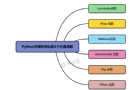
Use machine learning library to realize larger and better neural network , for example TensorFlow、Keras and PyTorch;
Implement neural network in browser ;
Other types of activation functions ;
Other types of optimizers ;
Learn convolutional neural networks , This has revolutionized the field of computer vision ;
Learn recurrent neural networks , Common language naturallanguageprocessing ;
Attach a piece of code
#!/usr/bin/pyton3
import numpy as np
import matplotlib.pyplot as plt
# Activation Function
def sigmoid(x):
return 1 / (1 + np.exp(-x))
# Neural Unit
class Perceptron(object):
def __init__(self, input_size: int, initializer: list = None, activation_func: str = None):
# W[0] is the bias
self.input_size = input_size
# W is parameters of Perceptron
self.n_W = self.input_size + 1
self.W = np.random.uniform(low=0.0, high=1.0, size=self.n_W)
# X is the input vector of Perceptron
self.X = None
self.output = 0.0
self.delta_W = np.array([0] * self.n_W, dtype=np.float)
self.delta_X = np.array([0] * input_size, dtype=np.float)
self.activation_func = activation_func
if initializer:
assert len(initializer) == self.n_W
self.W = initializer
def forward(self, X):
assert len(X) == self.input_size
self.X = np.array(X, dtype=float)
y = np.sum(self.W[1:] * self.X) + self.W[0]
if self.activation_func == 'sigmoid':
self.output = sigmoid(y)
else:
self.output = y
return self.output
def update(self, lr):
self.W = self.W + lr * self.delta_W
self.delta_W = np.array([0] * self.n_W, dtype=np.float)
def __call__(self, X):
return self.forward(X)
# Neural Layer
class Layer(object):
def __init__(self, input_size: int, output_size: int, activation_func='sigmoid', lr=0.1):
self.input_size = input_size
self.output_size = output_size
self.net = np.array(
[Perceptron(input_size=input_size, activation_func=activation_func) for _ in range(output_size)])
self.activation_func = activation_func
self.inputs = np.array([0] * input_size, dtype=np.float)
self.lr = lr
self.outputs = np.array([0] * output_size, dtype=np.float)
def forward(self, X):
self.inputs = np.array(X, dtype=np.float)
self.outputs = np.array([p(X) for p in self.net])
return self.outputs
def __call__(self, X):
return self.forward(X)
def backward(self, delta_outputs):
assert len(delta_outputs) == len(self.net)
for idx in range(self.output_size):
delta_output = delta_outputs[idx]
p = self.net[idx]
o = self.outputs[idx]
if self.activation_func == 'sigmoid':
# W0 is the bias
p.delta_W = delta_output * o * (1 - o) * np.array([1] + list(p.X)) # expand X for W_0
p.delta_X = delta_output * o * (1 - o) * p.W[1:]
else:
# linear
p.delta_W = delta_output * np.array([1] + list(p.X))
# W0 is the bias
p.delta_X = delta_output * p.W[1:]
def update(self):
for p in self.net:
p.update(self.lr)
if __name__ == '__main__':
# standard version ============================
samples = [[[-2, -1], 1],
[[25, 6], 0],
[[17, 4], 0],
[[-15, -6], 1]]
# training
layer1 = Layer(2, 10)
layer2 = Layer(10, 1, activation_func='')
for i in range(1000):
# iteration
print(f'iteration {
i}')
text_X = samples[3][0]
text_y_d = samples[3][1]
test_y = layer2(layer1((samples[3][0])))[0]
print(f'X:{
text_X}, y_d:{
text_y_d}, y:{
test_y}')
for X, y_d in samples:
# forward
y = layer2(layer1(X))[0]
# backward layer2 -> layer1
err = y_d - y # delta_outputs of layer 2
layer2.backward([err])
delta_outputs = np.array([0.0] * layer2.input_size, dtype=np.float) # delta_outputs of layer 1
for p in layer2.net:
delta_outputs += p.delta_X
layer1.backward(delta_outputs)
# update gradient
layer2.update()
layer1.update()
# result
for X, y_d in samples:
y = layer2(layer1(X))[0]
print(f'The final result: X:{
X}, y_d:{
y_d}, y:{
y}')
# # simple version ============================
# samples = [[[0, 1], 1],
# [[1, 0], -1]]
# # training
# layer1 = Layer(2, 1, activation_func='')
# for i in range(100):
# # iteration
# print(f'iteration {i}')
# for X, y_d in samples:
# # forward
# y = layer1(X)[0]
# # backward
# err = y_d - y
# layer1.backward([err])
# print(f'W:{layer1.net[0].W}')
# print(f'delta_W:{layer1.net[0].delta_W}')
# layer1.update()
# print(f'X:{X}, y_d:{y_d}, y:{y}')