Read gold ETF data
This paper uses machine learning method to predict the price of gold, one of the most important precious metals . We will create a linear regression model , The model from the past gold ETF (GLD) Get information from the price , And return to the next day's gold ETF Price forecast .GLD It is the largest direct investment in physical gold ETF.
The first thing to do is : Import all necessary Libraries .
# LinearRegression  Is a machine learning library for linear regression
from sklearn.linear_model import LinearRegression
# pandas  and  numpy  For data manipulation
import pandas as pd
import numpy as np
# matplotlib  and  seaborn  Used to draw graphics
import matplotlib.pyplot as plt
%matplotlib inline
plt.style.use('seaborn-darkgrid')
# yahoo Finance For retrieving data
import yfinance as yf
then , We read the past 12 Annual daily gold ETF Price data and store it in Df in . We delete irrelevant columns and use dropna() Function delete NaN value . then , We draw gold ETF Closing price .
Df = yf.download('GLD', '2008-01-01', '2020-6-22', auto_adjust=True)
Df = Df[['Close']]
Df = Df.dropna()
Df.Close.plot(figsize=(10, 7),color='r')
plt.ylabel("Gold ETF Prices")
plt.title("Gold ETF Price Series")
plt.show()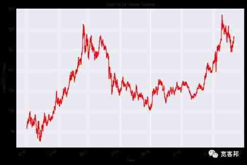
Define explanatory variables
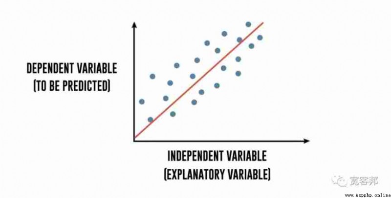
The explanatory variable is one that is manipulated to determine the next day's gold ETF Price variables . In short , They are what we want to use to predict gold ETF The characteristics of price .
The explanatory variable in this strategy is the past 3 Days and 9 Day moving average . We use dropna() Function delete NaN Store the characteristic value in X in .
however , You can go to X Add more you think about forecasting gold ETF Price is a useful variable . These variables can be technical indicators 、 other ETF The price of , For example, gold miners ETF (GDX) Or oil ETF (USO), Or US economic data .
Define the dependent variable
Again , The dependent variable depends on the value of the explanatory variable . In short , This is the gold we are trying to predict ETF Price . We will gold ETF Prices are stored in y in .
Df['S_3'] = Df['Close'].rolling(window=3).mean()
Df['S_9'] = Df['Close'].rolling(window=9).mean()
Df['next_day_price'] = Df['Close'].shift(-1)
Df = Df.dropna()
X = Df[['S_3', 'S_9']]
y = Df['next_day_price']
Split the data into training and test data sets
In this step , We split the prediction variables and output data into training data and test data . By pairing the input with the expected output , The training data is used to create a linear regression model .
The test data is used to estimate the training effect of the model .
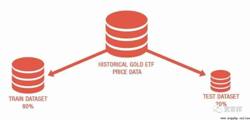
• front 80% Data for training , The remaining data is used to test
•X_train & y_train It's the training data set
•X_test & y_test It's a test data set
t = .8
t = int(t*len(Df))
X_train = X[:t]
y_train = y[:t]
X_test = X[t:]
y_test = y[t:]
Create a linear regression model
We will now create a linear regression model . however , What is linear regression ?
If we try to catch “x” and “y” The mathematical relationship between variables , By fitting a line to the scatter plot ,“ best ” according to “x” The observations explain “y” The observations , So this equation x and y The relationship between is called linear regression analysis .
To further decompose , Regression uses independent variables to explain the changes of dependent variables . The dependent variable “y” Is the variable you want to predict . The independent variables “x” Is the explanatory variable you use to predict the dependent variable . The following regression equation describes this relationship :
Y = m1 * X1 + m2 * X2 + C
Gold ETF price = m1 * 3 days moving average + m2 * 15 days moving average + c
Then we use the fitting method to fit the independent variable and dependent variable (x and y) To generate regression coefficients and constants .
linear = LinearRegression().fit(X_train, y_train)
print("Linear Regression model")
print("Gold ETF Price (y) = %.2f * 3 Days Moving Average (x1) \
+ %.2f * 9 Days Moving Average (x2) \
+ %.2f (constant)" % (linear.coef_[0], linear.coef_[1], linear.intercept_))
Output linear regression model :
gold ETF Price (y) = 1.20 * 3 Day moving average (x1) + -0.21 * 9 Day moving average (x2) + 0.43( constant )
Forecast gold ETF Price
Now? , It's time to check if the model works in the test dataset . We use a linear model created using the training data set to predict gold ETF Price . The prediction method finds a given explanatory variable X Of gold ETF Price (y).
predicted_price = linear.predict(X_test)
predicted_price = pd.DataFrame(
    predicted_price, index=y_test.index, columns=['price'])
predicted_price.plot(figsize=(10, 7))
y_test.plot()
plt.legend(['predicted_price', 'actual_price'])
plt.ylabel("Gold ETF Price")
plt.show()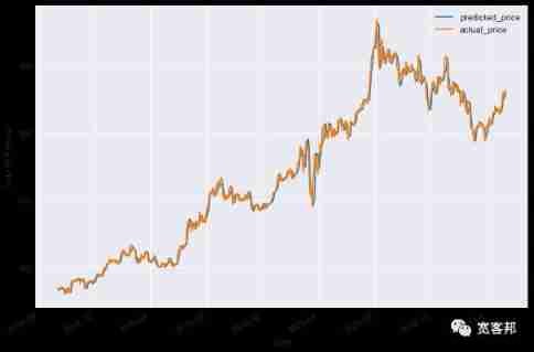
The picture shows gold ETF The predicted price and the actual price .
Now? , Let's use score() Function to calculate goodness of fit .
r2_score = linear.score(X[t:], y[t:])*100
float("{0:.2f}".format(r2_score))
Output :
99.21
It can be seen that , Model R Square is 99.21%.R Square is always between 0 and 100% Between . near 100% The score shows that the model well explains gold ETF The price of .
Plot cumulative income
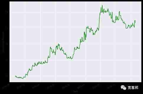
Let's calculate the cumulative return of this strategy to analyze its performance .
The calculation steps of cumulative income are as follows :
• Generate daily percentage change in gold price
• When the forecast price of the next day is higher than that of the current day , Create a to “1” Indicates a buying signal
• Calculate the strategic return by multiplying the daily percentage change by the trading signal .
• Last , We will draw a cumulative income chart
gold = pd.DataFrame()
gold['price'] = Df[t:]['Close']
gold['predicted_price_next_day'] = predicted_price
gold['actual_price_next_day'] = y_test
gold['gold_returns'] = gold['price'].pct_change().shift(-1)
gold['signal'] = np.where(gold.predicted_price_next_day.shift(1) < gold.predicted_price_next_day,1,0)
gold['strategy_returns'] = gold.signal * gold['gold_returns']
((gold['strategy_returns']+1).cumprod()).plot(figsize=(10,7),color='g')
plt.ylabel('Cumulative Returns')
plt.show()
Output is as follows :
We will also calculate Sharpe ratio :
sharpe = gold['strategy_returns'].mean()/gold['strategy_returns'].std()*(252**0.5)
'Sharpe Ratio %.2f' % (sharpe)
Output is as follows :
'Sharpe Ratio 1.06'
Forecast daily prices
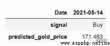
You can use the following code to predict the price of gold , And give us what we should buy GLD Or a trading signal not to hold a position :
import datetime as dt
current_date = dt.datetime.now()
data = yf.download('GLD', '2008-06-01', current_date, auto_adjust=True)
data['S_3'] = data['Close'].rolling(window=3).mean()
data['S_9'] = data['Close'].rolling(window=9).mean()
data = data.dropna()
data['predicted_gold_price'] = linear.predict(data[['S_3', 'S_9']])
data['signal'] = np.where(data.predicted_gold_price.shift(1) < data.predicted_gold_price,"Buy","No Position")
data.tail(1)[['signal','predicted_gold_price']].T
Output is as follows :
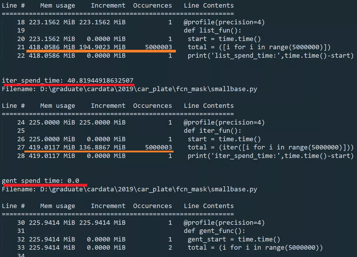
 In Python, the iteration generator yield can be used to reduce memory consumption
stay python In the encoding fo