RIGHT Example:
names = ['孫悟空', '李元芳', '白起', '狄仁傑', '達摩']
courses = ['語文', '數學', '英語']
import random
scores = [[random.randrange(60, 101) for _ in range(3)] for _ in range(5)]
print(scores)
# [[100, 97, 76], [91, 79, 66], [84, 78, 71], [87, 81, 96], [73, 71, 88]]
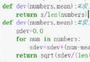
def mean(nums):
"""求均值"""
return sum(nums) / len(nums)
def variance(nums):
"""求方差"""
mean_value = mean(nums)
return mean([(num - mean_value) ** 2 for num in nums])
def stddev(nums):
"""求標准差"""
return variance(nums) ** 0.5
# 統計每個學生的考試平均分
for idx, name in enumerate(names):
temp = scores[idx]
avg_score = mean(temp)
print(f'{
name}考試平均分為:{
avg_score:.1f}分')
''' 孫悟空考試平均分為:91.0分 李元芳考試平均分為:78.7分 白起考試平均分為:77.7分 狄仁傑考試平均分為:88.0分 達摩考試平均分為:77.3分 '''
# 統計每門課的最高分、最低分、標准差
for idx, course in enumerate(courses):
temp = [scores[i][idx] for i in range(len(names))]
max_score, min_score = max(temp), min(temp)
print(f'{
course}成績最高分:{
max_score}分')
print(f'{
course}成績最低分:{
min_score}分')
print(f'{
course}成績標准差:{
stddev(temp):.1f}分')
''' 語文成績最高分:100分 語文成績最低分:73分 語文成績標准差:8.8分 數學成績最高分:97分 數學成績最低分:71分 數學成績標准差:8.6分 英語成績最高分:96分 英語成績最低分:66分 英語成績標准差:11.1分 '''
# 將學生及其考試成績以行的方式輸出(按平均分從高到低排序)
results = {
name: temp for name, temp in zip(names, scores)}
sorted_keys = sorted(results, key=lambda x: mean(results[x]), reverse=True)
for key in sorted_keys:
verbal, math, english = results[key]
print(f'{
key}:\t{
verbal}\t{
math}\t{
english}')
''' 孫悟空: 100 97 76 狄仁傑: 87 81 96 李元芳: 91 79 66 白起: 84 78 71 達摩: 73 71 88 '''
Python數據分析三大神器
import numpy as np
import pandas as pd
import matplotlib.pyplot as plt
# 將list處理成ndarray對象
scores = np.array(scores)
print(scores)
''' array([[100, 97, 76], [ 91, 79, 66], [ 84, 78, 71], [ 87, 81, 96], [ 73, 71, 88]]) '''
# 查看數據類型
type(scores)
# numpy.ndarray
# 按橫向(學生)求平均值
np.round(scores.mean(axis=1), 1)
# array([91. , 78.7, 77.7, 88. , 77.3])
# 按豎向(學科)求最高分、最低分、標准差
scores.max(axis=0)
# array([100, 97, 96])
scores.min(axis=0)
# array([73, 71, 66])
np.round(scores.std(axis=0), 1)
# array([ 8.8, 8.6, 11.1])
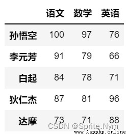
scores_df = pd.DataFrame(data=scores, columns=courses, index=names)
scores_df
效果圖:
# 計算平均分
np.round(scores_df.mean(axis=1), 1)
''' 孫悟空 91.00000 李元芳 78.66875 白起 77.66875 狄仁傑 88.00000 達摩 77.33125 dtype: float64 '''
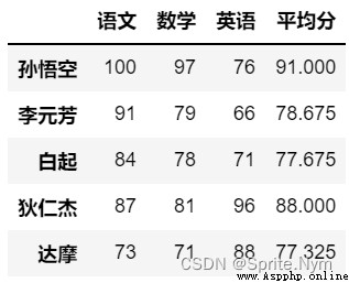
# 添加平均分列到表中
scores_df['平均分']= scores_df.mean(axis=1)
scores_df
效果圖:
# 寫入Excel文件
scores_df.to_excel('考試成績.xlsx')
# 改plt字體
plt.rcParams['font.sans-serif'] = ['KaiTi']
plt.rcParams['axes.unicode_minus'] = False
# 將生成的圖表改成矢量圖
%config InlineBackend.figure_format='svg'
# 生成柱狀圖
scores_df.plot(kind='bar', y=['語文','數學','英語'])
# 旋轉橫軸的刻度
plt.xticks(rotation=0)
# 保存圖表
plt.savefig('成績柱狀圖.svg')
# 顯示圖表
plt.show()
效果圖: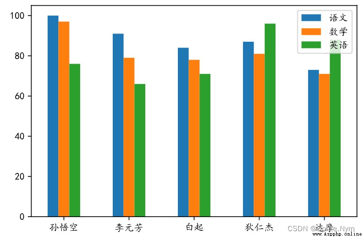
# 求學科最高分、最低分、平均分
scores_df.max()
''' 語文 100.0 數學 97.0 英語 96.0 平均分 91.0 dtype: float64 '''
scores_df.min()
''' 語文 73.0 數學 71.0 英語 66.0 平均分 77.3 dtype: float64 '''
scores_df.std()
''' 語文 9.874209 數學 9.602083 英語 12.361230 平均分 6.461656 dtype: float64 '''
# 方法一:通過array函數將list處理成ndarray對象
array1 = np.array([1, 2, 10, 20, 100])
array1
# array([ 1, 2, 10, 20, 100])
type(array1)
# numpy.ndarray
# 方法二:指定一個范圍創建數組對象
array2 = np.arange(1, 100, 2)
array2
''' array([ 1, 3, 5, 7, 9, 11, 13, 15, 17, 19, 21, 23, 25, 27, 29, 31, 33,35, 37, 39, 41, 43, 45, 47, 49, 51, 53, 55, 57, 59, 61, 63, 65, 67, 69, 71, 73, 75, 77, 79, 81, 83, 85, 87, 89, 91, 93, 95, 97, 99]) '''
# 方法三:指定范圍和元素的個數創建數組對象
array3 = np.linspace(-5, 5, 101)
array3
''' array([-5. , -4.9, -4.8, -4.7, -4.6, -4.5, -4.4, -4.3, -4.2, -4.1, -4. , -3.9, -3.8, -3.7, -3.6, -3.5, -3.4, -3.3, -3.2, -3.1, -3. , -2.9, -2.8, -2.7, -2.6, -2.5, -2.4, -2.3, -2.2, -2.1, -2. , -1.9, -1.8, -1.7, -1.6, -1.5, -1.4, -1.3, -1.2, -1.1, -1. , -0.9, -0.8, -0.7, -0.6, -0.5, -0.4, -0.3, -0.2, -0.1, 0. , 0.1, 0.2, 0.3, 0.4, 0.5, 0.6, 0.7, 0.8, 0.9, 1. , 1.1, 1.2, 1.3, 1.4, 1.5, 1.6, 1.7, 1.8, 1.9, 2. , 2.1, 2.2, 2.3, 2.4, 2.5, 2.6, 2.7, 2.8, 2.9, 3. , 3.1, 3.2, 3.3, 3.4, 3.5, 3.6, 3.7, 3.8, 3.9, 4. , 4.1, 4.2, 4.3, 4.4, 4.5, 4.6, 4.7, 4.8, 4.9, 5. ]) '''
# 方法四:用隨機生成元素的方法創建數組對象
# 隨機小數
array4 = np.random.random(10)
array4
''' array([0.74861994, 0.80263292, 0.54287411, 0.99088428, 0.27465232, 0.4421258 , 0.34908231, 0.39729076, 0.11863797, 0.37728455]) '''
# 隨機整數
array5 = np.random.randint(1, 10)
array5
# 5
# 隨機正態分布
array6 = np.random.normal(0, 1, 50000)
array6
''' array([-1.24165108, -0.07314869, -1.37729185, ..., -1.00691177, 0.19568883, 0.43887128]) '''
# 生成直方圖
plt.hist(array6, bins=24)
plt.show()
效果圖: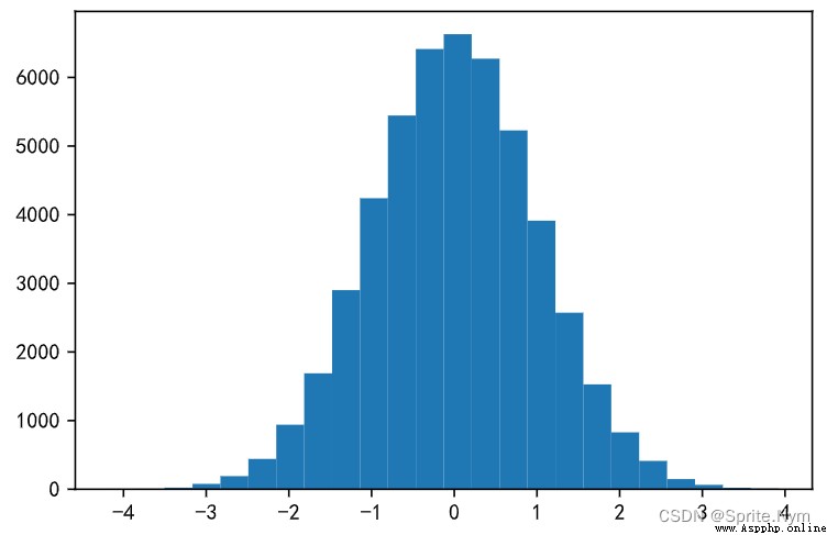
# 方法一:通過array函數將嵌套列表處理成二維數組
array8 = np.array(([1, 2, 3], [4, 5, 5], [7, 8, 9]))
array8
''' array([[1, 2, 3], [4, 5, 5], [7, 8, 9]]) '''
# 方法二:通過對一維數組調形變成二維數組
temp= np.arange(1, 11)
array9 = temp.reshape((5, 2))
array9
''' array([[ 1, 2], [ 3, 4], [ 5, 6], [ 7, 8], [ 9, 10]]) '''
# 方法三;通過生成隨機元素創建二維數組
array10 = np.random.randint(60, 101, (5, 3))
array10
''' array([[71, 91, 67], [95, 71, 96], [90, 91, 92], [67, 83, 74], [95, 78, 60]]) '''
# 方法四:創建全0、全1、指定值的二維數組
array11 = np.zeros((5, 4), dtype='i8')
array11
''' array([[0, 0, 0, 0], [0, 0, 0, 0], [0, 0, 0, 0], [0, 0, 0, 0], [0, 0, 0, 0]], dtype=int64) '''
array12 = np.ones((5, 4), dtype='i8')
array12
''' array([[1, 1, 1, 1], [1, 1, 1, 1], [1, 1, 1, 1], [1, 1, 1, 1], [1, 1, 1, 1]], dtype=int64) '''
array13 = np.full((5, 4), 100)
array13
''' array([[100, 100, 100, 100], [100, 100, 100, 100], [100, 100, 100, 100], [100, 100, 100, 100], [100, 100, 100, 100]]) '''
# 方法五:創建單位矩陣
array14 = np.eye(5)
array14
''' array([[1., 0., 0., 0., 0.], [0., 1., 0., 0., 0.], [0., 0., 1., 0., 0.], [0., 0., 0., 1., 0.], [0., 0., 0., 0., 1.]]) '''
array10
''' array([[71, 91, 67], [95, 71, 96], [90, 91, 92], [67, 83, 74], [95, 78, 60]]) '''
# 取指定元素
array10[1][2]
# 96
array10[1, 2]
# 96
# 取部分元素
array10[:3, :2]
''' array([[71, 91], [95, 71], [90, 91]]) '''
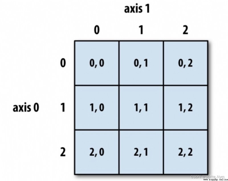
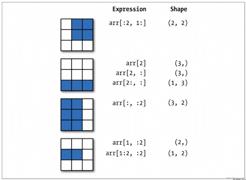
總結:對多維數組的操作中,每做一次索引降一次維,而做切片不會降維。
# 花式索引(fancy index)
array2[[0, 1, 2, -3, -2, -1, -10]]
# array([ 1, 3, 5, 95, 97, 99, 81])
array10[[0, 1, 4], [0, 1, 2]]
# array([71, 71, 60])
# 布爾索引
array1[[False, True, False, True, False]]
# array([ 2, 20], dtype=uint64)
array2[array2 > 80]
# array([81, 83, 85, 87, 89, 91, 93, 95, 97, 99])
array16 = np.arange(1, 10)
array16[array16 % 2 !=0]
# array([1, 3, 5, 7, 9])
array16[(array16 > 5) & (array16 % 2 != 0)]
# array([7, 9])
array16[(array16 > 5) | (array16 % 2 != 0)]
# array([1, 3, 5, 6, 7, 8, 9])
array16[(array16 > 5) | ~(array16 % 2 != 0)]
# array([2, 4, 6, 7, 8, 9])
array10[array10 > 80]
# array([91, 95, 96, 90, 91, 92, 83, 95])
array1 = np.random.randint(10, 50, 10)
array1
# 求和
array1.sum
np.sum(array1)
# 求平均
array1.mean()
np.mean(array1)
# 求中位數
np.median(array1)
# 求最大值最小值
array1.max()
np.amax(array1)
array1.min()
np.amin(array1)
# 求極差(全距)
array1.ptp()
np.ptp(array1)
# 求方差
array1.var
np.var(array1)
# 求標准差
array1.std
np.std(array1)
# 求累計和
array1.cumsum()
np.cumsum(array1)


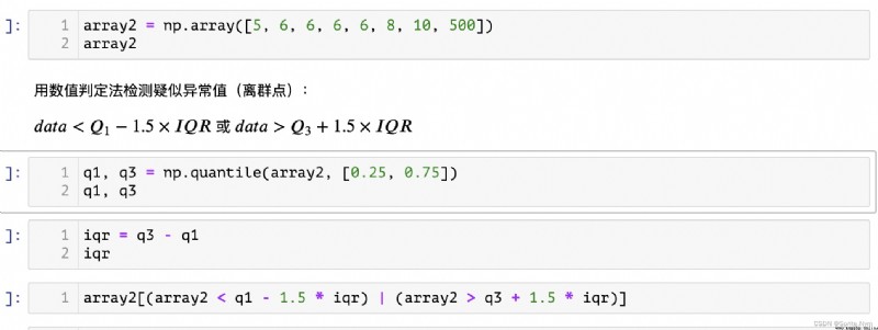
def outliers_by_iqr(t_array, lower_points = 0.25, upper_points = 0.75, whis = 1.5):
"""iqr找異常值"""
q1, q3 = np.quantile(t_array, [lower_points, upper_points])
iqr = q3 - q1
return t_array[(t_array < q1 - whis * iqr)|(t_array > q3 + whis * iqr)]
# 測試
array2[-1] = 15
outliers_by_iqr(array2)
# array([15])
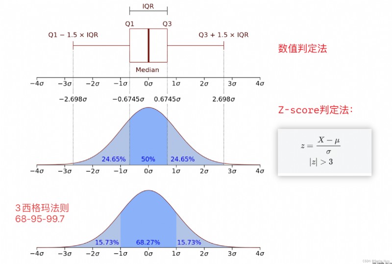
def outliers_by_zscore(array, threshold=3):
"""Z-score判定法檢測離群點"""
mu, sigma = array.mean(), array.std()
return array[np.abs((array - mu) / sigma) > threshold]
# 把數組改長點,以使500顯得突兀
# repeat()(會把相同元素放在一起)和tile()(按原本的順序重復)
temp = np.repeat(array2[:-1], 100)
# append()和insert()添加
temp = np.append(temp, array2[-1])
temp = np.insert(temp, 0, array2[-1])
temp
outliers_by_zscore(temp)
# array([500, 500])
判斷數組中是否所有元素都是True/判斷數組是否有True的元素。
拷貝數組,並將數組中的元素轉換為指定的類型。
array5 = array3.astype(np.float64)
array5.dtype
# dtype('float64')
保存數組到文件中,可以通過NumPy中的load()函數從保存的文件中家在數據創建數組。
序列化:把對象處理成字符串(str)或字節串(bytes) —> 串行化/腌鹹菜
反序列化:把字符串或字節串還原成對象 —> 反串行化
json模塊:dump / dumps / load / loads —> 通用,跨語言
pickle模塊:dump / dumps / load / loads —> 私有協議,其他語言無法反序列化
# 保存
with open('array3', 'wb') as file:
array3.dump(file)
# 讀取
with open('array3', 'rb') as file:
array6 = np.load(file, allow_pickle=True)
array6
向數組中填充指定的元素。即數組中元素全部變成指定元素。
將多維數組扁平化成一維數組
array7 = np.arange(1, 11).reshape(5, 2)
array7
''' array([[ 1, 2], [ 3, 4], [ 5, 6], [ 7, 8], [ 9, 10]]) '''
array7.flatten('C')
# array([ 1, 2, 3, 4, 5, 6, 7, 8, 9, 10])
array7.flatten('F')
# array([ 1, 3, 5, 7, 9, 2, 4, 6, 8, 10])
返回非0元素的索引
對數組中的元素做四捨五入操作。
array8 = np.random.randint(1, 100, 10)
array8
# array([55, 98, 48, 98, 38, 5, 35, 36, 39, 87])
# 返回排序後的新數組
np.sort(array8)
# array([ 5, 35, 36, 38, 39, 48, 55, 87, 98, 98])
array8
# array([55, 98, 48, 98, 38, 5, 35, 36, 39, 87])
# 在原始數組上就地排序
array8.sort()
# 無返回值
array8
# array([ 8, 10, 12, 27, 28, 43, 45, 57, 65, 98])
交換數組指定的軸。
# 對於二維數組,transpose相當於實現了矩陣的轉置
array7.transpose()
''' array([[ 1, 3, 5, 7, 9], [ 2, 4, 6, 8, 10]]) '''
# swapaxes交換指定的兩個軸,順序無所謂
array7.swapaxes(0, 1)
''' array([[ 1, 3, 5, 7, 9], [ 2, 4, 6, 8, 10]]) '''
將數組轉成Python中的list。不改變原數組。
array7.tolist()
# [[1, 2], [3, 4], [5, 6], [7, 8], [9, 10]]
去重。
array9 = np.array([1,1,1,1,2,2,2,3,3,3])
array9
# array([1, 1, 1, 1, 2, 2, 2, 3, 3, 3])
np.unique(array9)
# array([1, 2, 3])
array10 = np.array([[1,1,1], [2,2,2]])
array10
''' array([[1, 1, 1], [2, 2, 2]]) '''
array11 = np.array([[3,3,3,], [4,4,4,]])
array11
''' array([[3, 3, 3], [4, 4, 4]]) '''
# 水平方向(沿著1軸方向)的堆疊
np.hstack((array10, array11))
''' array([[1, 1, 1, 3, 3, 3], [2, 2, 2, 4, 4, 4]]) '''
# 垂直方向(沿著0軸方向)的堆疊
np.vstack((array10, array11))
''' array([[1, 1, 1], [2, 2, 2], [3, 3, 3], [4, 4, 4]]) '''
# 沿著指定軸堆疊並升維
np.stack((array10, array11), axis=0)
''' array([[[1, 1, 1], [2, 2, 2]], [[3, 3, 3], [4, 4, 4]]]) '''
np.stack((array10, array11), axis=1)
''' array([[[1, 1, 1], [3, 3, 3]], [[2, 2, 2], [4, 4, 4]]]) '''
array12 = np.concatenate((array10, array11), axis=0)
array12
''' array([[1, 1, 1], [2, 2, 2], [3, 3, 3], [4, 4, 4]]) '''
array13 = np.concatenate((array10, array11), axis=1)
array13
''' array([[1, 1, 1, 3, 3, 3], [2, 2, 2, 4, 4, 4]]) '''
# 垂直方向(沿著0軸方向)的拆分
np.vsplit(array12, 2)
''' [array([[1, 1, 1], [2, 2, 2]]), array([[3, 3, 3], [4, 4, 4]])] '''
np.vsplit(array12, 4)
''' [array([[1, 1, 1]]), array([[2, 2, 2]]), array([[3, 3, 3]]), array([[4, 4, 4]])] '''
# 水平方向(沿著1軸方向)的拆分
np.hsplit(array12, 3)
''' [array([[1], [2], [3], [4]]), array([[1], [2], [3], [4]]), array([[1], [2], [3], [4]])] '''
# 沿著指定軸拆分
np.split(array13, 2)
''' [array([[1, 1, 1, 3, 3, 3]]), array([[2, 2, 2, 4, 4, 4]])] '''
np.split(array13, 3, axis=1)
''' [array([[1, 1], [2, 2]]), array([[1, 3], [2, 4]]), array([[3, 3], [4, 4]])] '''
# 按照指定的條件從數組中抽取元素(類似於布爾索引)
np.extract(array14 <= 50, array14)
# array([19, 23, 50])
array14[array14 <= 50]
# array([19, 23, 50])
# 按照條件列表處理數組中的元素得到新的數組(多條件)
np.select([array14 % 2 == 0, array14 % 2 != 0], [array14 / 2, array14 ** 2])
# array([ 361., 9025., 38., 529., 25.])
# 按照條件數組中的元素得到新的數組(單條件)
np.where(array14 % 2 == 0, array14, 0)
# array([ 0, 0, 76, 0, 50])
從左到右,從上到下循環填充
array15 = np.arange(1, 10).reshape((3, 3))
array15
''' array([[1, 2, 3], [4, 5, 6], [7, 8, 9]]) '''
# 調整數組的大小
np.resize(array15, (4, 4))
''' array([[1, 2, 3, 4], [5, 6, 7, 8], [9, 1, 2, 3], [4, 5, 6, 7]]) '''
# 替換數組中指定索引的元素
np.put(array15, 5, 100)
array15
''' array([[ 1, 2, 3], [ 4, 5, 100], [ 7, 8, 9]]) '''
np.put(array15, [1, 2], 100)
array15
''' array([[ 1, 100, 100], [ 4, 5, 100], [ 7, 8, 9]]) '''
# 替換數組中滿足條件的元素
np.place(array15, array15 == 100, [2, 3])
array15
''' array([[1, 2, 3], [4, 5, 2], [7, 8, 9]]) '''
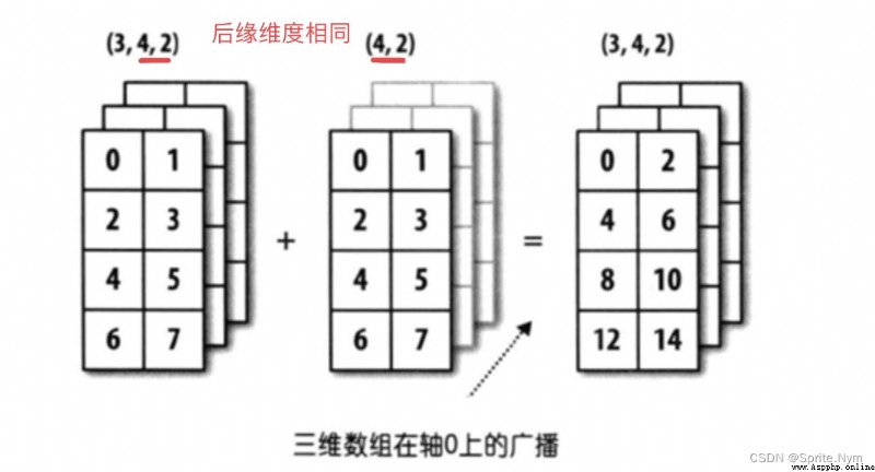
前提條件(必須滿足其中一個):
兩個數組的後緣維度(shape屬性從後往前看)相同。
兩個數組的後緣維度不同,但是其中一個維度為1。
滿足廣播機制是為了沿著缺失的軸或者沿著維度1的軸廣播自己,最終讓形狀變得一致。
# 滿足條件1:
array16 = np.arange(1, 16).reshape(5, 3)
array17 = np.array([[1, 1, 1]])
array16 + array17
''' array([[ 2, 3, 4], [ 5, 6, 7], [ 8, 9, 10], [11, 12, 13], [14, 15, 16]]) '''
# 還是滿足條件1:
array18 = np.random.randint(1, 18, (3, 4, 2))
array18
''' array([[[ 2, 11], [17, 16], [ 2, 6], [ 3, 13]], [[ 6, 17], [15, 4], [ 2, 2], [ 9, 6]], [[ 8, 4], [ 5, 9], [15, 11], [ 6, 17]]]) '''
array19 = np.random.randint(1, 10, (4, 2))
array19
''' array([[7, 5], [1, 7], [2, 7], [6, 5]]) '''


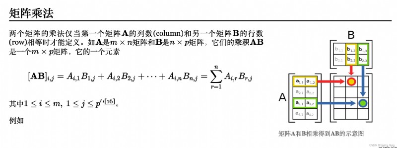
A ⋅ B = ∑ a i b i A \cdot B = \sum a_ib_i \\ A⋅B=∑aibi
A ⋅ B = ∣ A ∣ ∣ B ∣ c o s θ A \cdot B = |A||B|cos\theta A⋅B=∣A∣∣B∣cosθ
計算出來為標量
# 求點積
a = np.array([1, 2, 3])
b = np.array([2, 4, 6])
np.dot(a, b)
# 28,即1 * 2 + 2 * 4 + 3 * 6 = 28
# 求a的模
# linear algebra
np.linalg.norm(a)
# 求b的模
np.linalg.norm(b)
# 求a,b夾角的余弦值,進而得到a,b的相關度
np.dot(a, b) / np.linalg.norm(a) / np.linalg.norm(b)
# 1.0
# 創建矩陣
m1 = np.matrix('1 2; 3 4')
m1
''' matrix([[1, 2], [3, 4]]) '''
type(m1)
# numpy.matrix
# 獲取對應的數組對象
m1.A
''' array([[1, 2], [3, 4]]) '''
# 獲取對應的扁平化後的數組對象
m1.A1
''' array([1, 2, 3, 4]) '''
# 獲取轉置後的矩陣
m1.T
''' matrix([[1, 3], [2, 4]]) '''
m1.swapaxes(0, 1)
m1.transpose()
# 同理
# 獲取逆矩陣
m1.I
''' matrix([[-2. , 1. ], [ 1.5, -0.5]]) '''

A ⋅ A − 1 = I A \cdot A^{-1} = I A⋅A−1=I
m2 = np.matrix('1 0 2; -1 3 1')
m2
''' matrix([[ 1, 0, 2], [-1, 3, 1]]) '''
m3 = np.mat([[3, 1], [2, 1], [1, 0]])
m3
''' matrix([[3, 1], [2, 1], [1, 0]]) '''
m2 * m3
''' matrix([[5, 1], [4, 2]]) '''
# 通過嵌套列表或二維數組創建matrix對象
m4 = np.asmatrix(np.arange(1, 10).reshape((3, 3)))
m4
''' matrix([[1, 2, 3], [4, 5, 6], [7, 8, 9]]) '''
# determinent
# 計算矩陣的值
np.linalg.det(m4)
# 計算矩陣的秩
np.linalg.matrix_rank(m4)
array2 = m2.A
array2
''' array([[ 1, 0, 2], [-1, 3, 1]]) '''
array3 = m3.A
array3
''' array([[3, 1], [2, 1], [1, 0]]) '''
# 數組對象的矩陣乘法
array2 @ array3
''' array([[5, 1], [4, 2]]) '''
# 求逆矩陣
array1 = m1.A
np.linalg.inv(array1)
''' array([[-2. , 1. ], [ 1.5, -0.5]]) '''
{ x 1 + 2 x 2 + x 3 = 8 3 x 1 + 7 x 2 + 2 x 3 = 23 2 x 1 + 2 x 2 + x 3 = 9 \begin{cases} x_1 + 2x_2 + x_3 = 8 \\ 3x_1 + 7x_2 + 2x_3 = 23 \\ 2x_1 + 2x_2 + x_3 = 9 \end{cases} ⎩⎪⎨⎪⎧x1+2x2+x3=83x1+7x2+2x3=232x1+2x2+x3=9
A ⋅ x = b A \cdot x = b A⋅x=b
A = np.array([[1, 2, 1], [3, 7, 2], [2, 2, 1]])
b = np.array([8, 23, 9]).reshape(-1, 1)
C = np.hstack((A, b))
C
''' array([[ 1, 2, 1, 9], [ 3, 7, 2, 23], [ 2, 2, 1, 9]]) '''
np.linalg.matrix_rank(A)
# 3
np.linalg.matrix_rank(C)
# 3
A ⋅ x = b A − 1 ⋅ A ⋅ x = A − 1 ⋅ b I ⋅ x = A − 1 ⋅ b x = A − 1 ⋅ b A \cdot x = b \\ A^{-1} \cdot A \cdot x = A^{-1} \cdot b \\ I \cdot x = A^{-1} \cdot b \\ x = A^{-1} \cdot b \\ A⋅x=bA−1⋅A⋅x=A−1⋅bI⋅x=A−1⋅bx=A−1⋅b
# 用上面的公式解線性方程組
np.linalg.inv(A) @ b
''' array([[1.], [2.], [3.]]) '''
# 解線性方程組
np.linalg.solve(A, b)
''' array([[1.], [2.], [3.]]) '''
# 下載機器學習模塊
pip install scikit-learn
import warnings
warnings.filterwarnings('ignore')
from sklearn.datasets import load_boston
# 加載波士頓房價數據集
datasets = load_boston()
# 查看datasets屬性
dir(datasets)
# ['DESCR', 'data', 'data_module', 'feature_names', 'filename', 'target']
# 打印內容描述
print(datasets.DESCR)
# 內容太多不予展示
# 打印影響因素數據
datasets.data
# 內容太多不予展示
# 查看數據類型
type(datasets.data)
# numpy.ndarray
# 查看shape
datasets.data.shape
# (506, 13)
# 查看影響因素名
datasets.feature_names
''' array(['CRIM', 'ZN', 'INDUS', 'CHAS', 'NOX', 'RM', 'AGE', 'DIS', 'RAD', 'TAX', 'PTRATIO', 'B', 'LSTAT'], dtype='<U7') '''
# 獲得房價數據
y = datasets.target
y.shape
# (506,)
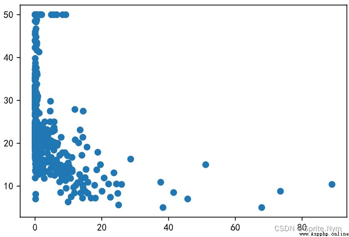
# 獲得犯罪率數據
x1 = datasets.data[:, 0]
x1.shape
# (506,)
# 計算犯罪率和房價相關系數
np.corrcoef(x1, y)
''' array([[ 1. , -0.38830461], [-0.38830461, 1. ]]) '''
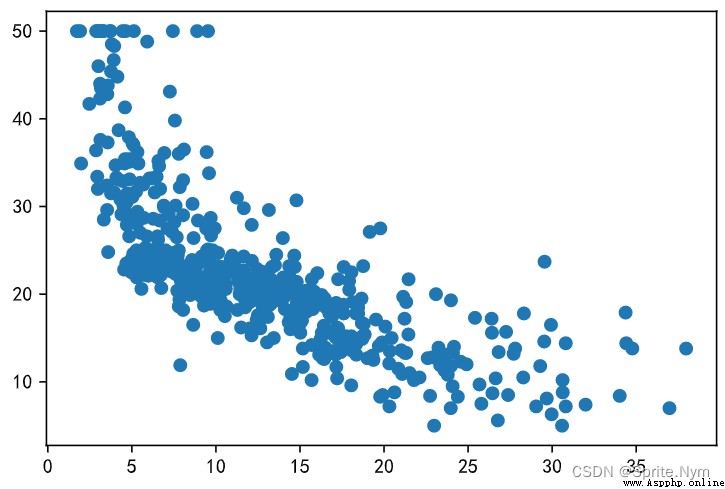
# 獲得低收入群體數據
x2 = datasets.data[:, -1]
x2.shape
# (506,)
# 計算低收入群體與房價相關系數
np.corrcoef(x2, y)
''' array([[ 1. , -0.73766273], [-0.73766273, 1. ]]) '''
# 後面相同的例子省略
# 畫散點圖
plt.scatter(x1, y)
plt.scatter(x2, y)
# 得到x:平均房間數數據,y:房價數據
x = datasets.data[:, 5]
y = datasets.target
# 將歷史數據存入字典
history_data = {
}
delta = 0
for room, price in zip(x, y):
if room not in history_data:
history_data[room] = price
else:
delta += 0.000001
history_data[room + delta] = price
len(history_data)
# 506
import heapq
def predicate_by_knn(room_num, k=5):
# 找到離目標數據最近的k個歷史數據
nearest_neighbors = heapq.nsmallest(k, history_data, key=lambda x:(x-room_num) ** 2)
# 計算歷史數據這些鍵對應的值的平均數
return round(np.mean([history_data[key] for key in nearest_neighbors]), 2)
# 調用函數試試
predicate_by_knn(6.125)
# 22.12
predicate_by_knn(5.525)
# 13.32
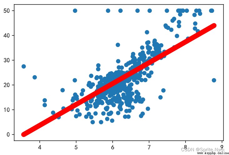
def get_loss(x, y, a, b):
"""損失函數"""
return np.mean((a * x + b - y) ** 2)
# 開始蒙特卡洛模擬,如果出現誤差更低的情況就記錄下來
min_loss = np.inf
best_a, best_b = None, None
for _ in range(10000):
a, b = np.random.random(2) * 200 - 100
curr_loss = get_loss(x, y, a, b)
if curr_loss < min_loss:
min_loss = curr_loss
best_a, best_b = a, b
print(a, b, min_loss)
print(best_a, best_b)
y_hat = best_a * x + best_b
# 畫圖看看
plt.scatter(x, y)
plt.plot(x, y_hat, color='red', linewidth=8)
# 定義出來根據擬合曲線求預測值的函數
def predicate_by_regression(room_num):
return round(best_a * room_num + best_b, 2)
# 調用函數試試
predicate_by_regression(5.525)
# 15
# 求a的偏導數
def partial_a(x, y, a, b):
return 2 * np.mean((y - a * x - b) * (-x))
# 求b的偏導數
def partial_b(x, y, a, b):
return 2 * np.mean(-y + a * x + b)
# 用梯度下降算法求a, b
a, b = 50, -50
delta = 0.013
for _ in range(1000):
a = a - partial_a(x, y, a, b) * delta
b = b - partial_b(x, y, a, b) * delta
print(get_loss(x, y, a, b))
print(best_a, best_b)
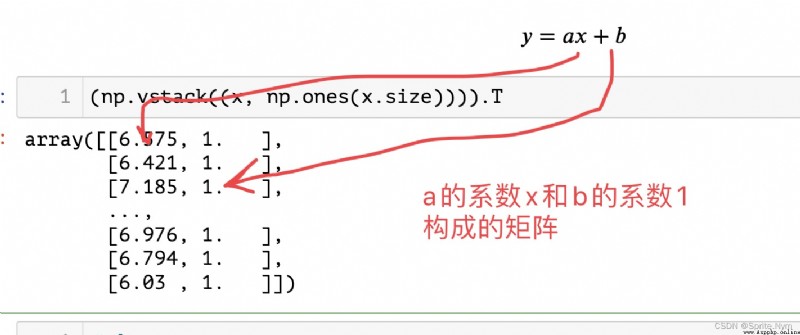
param1 = np.vstack((x, np.ones(x.size))).T
param1
param2 = y.reshape((-1, 1))
param2
# least square - 最小二乘解
results = np.linalg.lstsq(param1, param2)
results
''' (array([[ 9.10210898], [-34.67062078]]), array([22061.87919621]), 2, array([143.99484122, 2.46656609])) '''
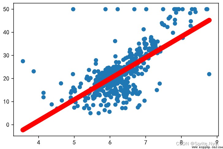
a, b = results[0].flatten()
a, b
# (9.102108981180313, -34.67062077643857)
y_hat = a * x + b
plt.scatter(x, y)
plt.plot(x, y_hat, color='red', linewidth=8)
# 創建Series對象
ser1 = pd.Series(data=[320, 180, 250, 220], index=[f'{
x}季度' for x in '1234'])
ser1
''' 1季度 320 2季度 180 3季度 250 4季度 220 dtype: int64 '''
# 通過字典創建series對象
ser2 = pd.Series(data={
'一季度': 320, '二季度': 180, '三季度': 250, '四季度': 220})
ser2
''' 一季度 320 二季度 180 三季度 250 四季度 220 dtype: int64 '''
# 普通索引
ser1['1季度']
# 320
ser2.一季度
# 320 (這種查詢方法不能改成1季度,因為數字不能開頭)
# 花式索引
ser1[['1季度', '3季度']]
''' 1季度 320 3季度 250 dtype: int64 '''
# 布爾索引
ser1[ser1 >= 200]
''' 1季度 320 3季度 250 4季度 220 dtype: int64 '''
ser1[1:3]
''' 2季度 180 3季度 250 dtype: int64 '''
# 用自己取的索引名來切片兩頭都可以取到
ser1['2季度': '3季度']
''' 2季度 180 3季度 250 dtype: int64 '''
# 獲取索引
ser2.index
# Index(['一季度', '二季度', '三季度', '四季度'], dtype='object')
# 獲取索引的值
ser2.index.values
# array(['一季度', '二季度', '三季度', '四季度'], dtype=object)
# 獲取數據
ser2.values
# array([320, 180, 250, 220], dtype=int64)
# 元素個數
ser2.size
# 4
# 元素是否唯一
ser2.is_unique
# True
# 有沒有空值
ser2.hasnans
# False
ser2['二季度'] = np.nan
ser2
''' 一季度 320.0 二季度 NaN 三季度 250.0 四季度 220.0 dtype: float64 '''
ser2.hasnans
# True
ser2['二季度'] = 280
ser2
# 280
# 數據是否單調遞增
ser2.is_monotonic_increasing
# False
# 數據是否單調遞減
ser2.is_monotonic_decreasing
# True
# 獲取描述性統計信息 - 集中趨勢
# 求和
print(ser2.sum())
# 求平均
print(ser2.mean())
# 中位數
print(ser2.median())
''' 1070.0 267.5 265.0 '''
# 眾數
print(ser2.mode())
''' 0 220.0 1 250.0 2 280.0 3 320.0 dtype: float64 '''
# 獲取描述性統計信息 - 離散趨勢
# 最大值和最小值
print(ser2.max())
print(ser2.min())
# 方差和標准差
print(ser2.var())
print(ser2.std())
print(np.var(ser2))
print(np.std(ser2))
# 上下四分位數
print(ser2.quantile(0.25))
print(ser2.quantile(0.75))
print(np.quantile(ser2, (0.25, 0.5, 0.75)))
''' 320 220 1825.0 42.720018726587654 1368.75 36.99662146737185 242.5 290.0 [242.5 265. 290. ] '''
# 直接獲取所有描述性統計信息
ser2.describe()
''' count 4.000000 mean 267.500000 std 42.720019 min 220.000000 25% 242.500000 50% 265.000000 75% 290.000000 max 320.000000 dtype: float64 '''
ser3 = pd.Series(['apple', 'banana', 'apple', 'pitaya', 'apple', 'pitaya', 'durian'])
ser3
''' 0 apple 1 banana 2 apple 3 pitaya 4 apple 5 pitaya 6 durian dtype: object '''
# 去重 ---> ndarray
ser3.unique()
# array(['apple', 'banana', 'pitaya', 'durian'], dtype=object)
# 不重復元素的個數
ser3.nunique()
# 4
# 元素重復的頻次(按頻次降序排列)
ser3.value_counts()
''' apple 3 pitaya 2 banana 1 durian 1 dtype: int64 '''
# 判斷元素是否重復
ser3.duplicated()
''' 0 False 1 False 2 True 3 False 4 True 5 True 6 False dtype: bool '''
# 布爾索引去重
ser3[~ser3.duplicated()]
''' 0 apple 1 banana 3 pitaya 6 durian dtype: object '''
# 去重 ---> Series
ser3.drop_duplicates()
''' 0 apple 1 banana 3 pitaya 6 durian dtype: object '''
# keep - 重復元素保留第一項還是最後一項,默認值first
ser3.drop_duplicates(keep='last')
''' 1 banana 4 apple 5 pitaya 6 durian dtype: object '''
# inplace - 是否就地進行操作
# True ---> 就地操作,不返回新的對象 ---> None
# False(默認值)---> 返回操作後的新對象 ---> Series
ser3.drop_duplicates(keep=False, inplace=True)
ser3
''' 1 banana 6 durian dtype: object '''
# 判斷空值
ser4.isnull()
''' 0 False 1 False 2 True 3 False 4 True dtype: bool '''
# 判斷非空值
ser4.notnull()
''' 0 True 1 True 2 False 3 True 4 False dtype: bool '''
# 通過布爾索引篩選非空值
ser4[ser4.notnull()]
''' 0 10.0 1 20.0 3 30.0 dtype: float64 '''
# 刪除指定的數據
ser4.drop(index=2)
''' 0 10.0 1 20.0 3 30.0 4 NaN dtype: float64 '''
ser4.drop(index=[2, 4])
''' 0 10.0 1 20.0 3 30.0 dtype: float64 '''
# 刪除空值(inplace=True,就地刪除)
ser4.dropna()
''' 0 10.0 1 20.0 3 30.0 dtype: float64 '''
# 填充空值
ser4.fillna(50)
''' 0 10.0 1 20.0 2 50.0 3 30.0 4 50.0 dtype: float64 '''
ser4.fillna(method='ffill')
''' 0 10.0 1 20.0 2 20.0 3 30.0 4 30.0 dtype: float64 '''
ser4.fillna(method='bfill')
''' 0 10.0 1 20.0 2 30.0 3 30.0 4 NaN dtype: float64 '''
# 前後都填充一次
ser4.fillna(method='ffill').fillna(method='bfill')
# 給索引排序
# ascending ---> 升序還是降序 ---> 默認值True,代表升序
ser1.sort_index(ascending=False)
''' 4季度 220 3季度 250 2季度 180 1季度 320 dtype: int64 '''
# 給值排序
ser1.sort_values(ascending=False)
''' 1季度 320 3季度 250 4季度 220 2季度 180 dtype: int64 '''
# Top-N
ser1.nlargest(3)
''' 1季度 320 3季度 250 4季度 220 dtype: int64 '''
ser1.nsmallest(2)
''' 2季度 180 4季度 220 dtype: int64 '''
# 例1:format對字符串批量處理
ser5 = pd.Series(['cat', 'dog', np.nan, 'rabbit'])
ser5
''' 0 cat 1 dog 2 NaN 3 rabbit dtype: object '''
ser5.map('I am a {}'.format, na_action='ignore')
''' 0 I am a cat 1 I am a dog 2 NaN 3 I am a rabbit dtype: object '''
# 例2:對數據批量處理
ser6 = pd.Series(np.random.randint(30, 80, 10))
ser6
''' 0 62 1 67 2 65 3 64 4 64 5 31 6 76 7 42 8 54 9 45 dtype: int32 '''
# 以下3種寫法都可以
def upgrade(score):
return score ** 0.5 * 10
# np.round(ser6.map(upgrade), 0)
# np.round(ser6.map(lambda x: x ** .5 * 10), 0)
np.round(ser6.apply(lambda x: x ** .5 * 10), 0)
''' 0 79.0 1 82.0 2 81.0 3 80.0 4 80.0 5 56.0 6 87.0 7 65.0 8 73.0 9 67.0 dtype: float64 '''
線性歸一化(標准化):
X i ′ = X i − X m i n X m a x − X m i n X_i' = \frac {X_{i} - X_{min}} {X_{max} - X_{min}} Xi′=Xmax−XminXi−Xmin
零均值歸一化(中心化):
X i ′ = X i − μ σ X_i' = \frac {X_{i} - \mu} {\sigma} Xi′=σXi−μ
# 例3:對數據進行歸一化
ser7 = pd.Series(data=np.random.randint(1, 10000, 10))
ser7
''' 0 9359 1 1222 2 2843 3 985 4 2478 5 3935 6 6838 7 1999 8 5907 9 9064 dtype: int32 '''
# 線性歸一化
x_min = ser7.min()
x_max = ser7.max()
ser7.map(lambda x: (x - x_min) / (x_max - x_min))
''' 0 1.000000 1 0.028302 2 0.221877 3 0.000000 4 0.178290 5 0.352281 6 0.698949 7 0.121089 8 0.587772 9 0.964772 dtype: float64 '''
# 零均值歸一化
miu = ser7.mean()
sigma = ser7.std()
ser7.map(lambda x: (x - miu) / sigma)
''' 0 1.646880 1 -1.090183 2 -0.544923 3 -1.169903 4 -0.667699 5 -0.177605 6 0.798885 7 -0.828822 8 0.485722 9 1.547650 dtype: float64 '''
ser7 = pd.Series(
data = np.random.randint(150, 550, 8),
index = [f'{
x}季度' for x in '11213434']
)
ser7
''' 1季度 322 1季度 440 2季度 348 1季度 256 3季度 242 4季度 483 3季度 401 4季度 448 dtype: int32 '''
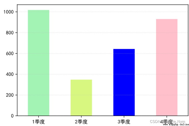
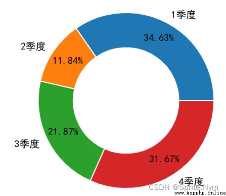
# 根據季度匯總數據繪制餅圖
# level = 0表示按0級索引分組
temp = ser7.groupby(level=0).sum()
temp
''' 1季度 1018 2季度 348 3季度 643 4季度 931 dtype: int32 '''
# 繪制柱狀圖
temp.plot(kind='bar', color=['#a3f3b4', '#D8F781', 'blue', 'pink'])
plt.xticks(rotation=0)
plt.grid(True, alpha=0.5, axis='y', linestyle=':')
plt.show()
# 繪制餅圖
temp.plot(kind='pie', autopct='%.2f%%', wedgeprops={

'edgecolor': 'w',
'width': 0.4,
}, pctdistance=0.8)
# 改y軸標簽
plt.ylabel('')
plt.show()
stuids = np.arange(1001, 1006)
courses = ['語文', '數學', '英語']
scores = np.random.randint(60, 101, (5, 3))
# 方法1:通過二維數組或嵌套創建DataFrame對象
df1 = pd.DataFrame(data = scores, columns = courses, index = stuids)
df1
# 方法2:通過字典創建DataFrame對象
scores = {

'語文': [62, 72, 93, 88, 93],
'數學': [95, 65, 86, 66, 87],
'英語': [66, 75, 82, 69, 82]
}
df2 = pd.DataFrame(data = scores, index = stuids)
df2
# 讀取CSV文件創建DataFrame對象
df4 = pd.read_csv(
'datas/2018年北京積分落戶數據.csv',
index_col='id', # 指定索引列
sep='#', # 指定分隔符
quotechar='`', # 包裹內容的字符
usecols=['id', 'name', 'score'], # 讀取哪些列
nrows=10, # 讀取的行數
skiprows=np.arange(1, 11) # 跳過的行數
# skiprows=lambda rn: rn > 0 and random.random() < 0.9 # 隨機跳過行數
)
df4
# 讀取CSV文件並創建成迭代器對象
df5_iter = pd.read_csv(
'datas/bilibili.csv',
encoding='gbk',
chunksize=10, # 10個內容1箱
iterator=True # 創建成迭代器對象
)
df5_iter
# 通過迭代器獲取DataFrame對象
next(df5_iter)
df6 = pd.read_excel('datas/全國旅游景點數據.xlsx')
df6
# 省略結果展示
df7 = pd.read_excel(
'datas/2020年銷售數據.xlsx',
sheet_name='data', # 要讀的表名
header=0, # 指定表頭位置
nrows=500,
skiprows=np.arange(1, 502)
)
df7
# 省略結果展示
df8 = pd.read_excel(
'datas/三國人物數據.xlsx',
sheet_name='全部人物數據',
header=0,
usecols=np.arange(0, 10)
)
df8
# 省略結果展示
# 創建conn對象
import pymysql
conn = pymysql.connect(host='47.104.31.138', port=3306,
user='guest', password='Guest.618',
database='hrs', charset='utf8mb4')
conn
# <pymysql.connections.Connection at 0x1c469df74f0>
# 或者創建engine對象
from sqlalchemy import create_engine
engine = create_engine('mysql+pymysql://guest:[email protected]/hrs')
engine
# 從engine對象或conn對象去提取數據
dept_df = pd.read_sql('select dno, dname, dloc from tb_dept', conn)
dept_df
# 省略結果展示
emp_df = pd.read_sql('select eno, ename, job, sal, comm, dno from tb_emp', engine)
emp_df
# 省略結果展示
from sqlalchemy import create_engine
engine = create_engine('mysql+pymysql://guest:[email protected]:3306/hrs')
engine
# 獲取部門表
dept_df = pd.read_sql('select dno, dname, dloc from tb_dept', engine)
dept_df
# 獲取員工表
emp_df = pd.read_sql('select eno, ename, job, sal, comm, dno from tb_emp', engine)
emp_df
# 用DataFrame的方法去內聯結
emp_df.merge(dept_df, how='inner', on='dno')
# 改列名後,兩表列名不再相等
dept_df.rename(columns={
'dno': 'deptno'}, inplace=True)
# 用left_on和right_on設置聯表條件
temp_df = emp_df.merge(dept_df, how='inner', left_on='dno', right_on='deptno')
temp_df
# 也可以用函數聯表
temp_df = pd.merge(emp_df, dept_df, how='inner',
left_on='dno', right_on='deptno')
temp_df
# 此時不會自動合並用於聯表的相同列,可以手動刪除
temp_df.drop(columns=['deptno', 'job'], inplace=True)
# 將deptno列改為索引列
dept_df = dept_df.set_index('deptno')
# 聯結條件是索引列時寫right_index=True
pd.merge(emp_df, dept_df, how='inner', left_on='dno', right_index=True)
import os
# ignore_index=True表示無視原來的編號重新編號
df1 = pd.concat([pd.read_csv(f'datas/jobs/{
i}') for i in os.listdir('datas/jobs')],
ignore_index=True)
df1.drop(columns=['uri', 'city'], inplace=True)
df1
# 1. 操作列
# 獲取指定列
df1['site']
# 計算不重復公司名數
df1['company_name'].nunique()
# 去重
df1['company_name'].drop_duplicates()
# 花式索引同時獲取多列
df1[['company_name', 'site', 'edu']]
# 布爾索引
df1[df1['edu']=='本科']
# 按索引列和列名同時取多行
df1.loc[[4, 7, 1]]
# 按自帶索引切片取多行
df1.iloc[1:5]
# 按索引列切片取多行
df1.loc[1:5]
# 2. 操作單元格
# 按索引列和列名鎖定單元格
df1.at[7, 'company_name']
# 按編號鎖定單元格
df1.iat[7, 0]
# 修改單元格
df1.iat[7, 0] = '川大資本家'
注意:iloc和loc、iat和at,不加i表示按行名和列名查,加了i表示按索引號順序查。
# 判斷是否是空值
emp_df.isnull()
# 判斷是否是非空值
emp_df.notnull()
# 刪除含空值的行(即沿著0軸刪)
emp_df.dropna()
# 刪除含空值的列(即沿著1軸刪)
emp_df.dropna(axis=1)
# 填充指定列的空值(由於每一列處理空值要求不同,所以一列列改)
emp_df['comm'] = emp_df['comm'].fillna(0).astype(np.int64)
emp_df
# 判斷重復
emp_df.duplicated('job')
# 去重
emp_df.drop_duplicates('job', keep='first')
# 獲取DataFrame對象的相關信息
ytb.info()
# 獲取DataFrame對象的前10行
ytb.head(10)
# 獲取DataFrame對象的後10行
ytb.tail(10)
案例:
# 不限制最大顯示列數
pd.set_option('display.max_column', None)
# 讀科比投籃數據表
kobe = pd.read_csv('datas/Kobe_data.csv', index_col='shot_id')
kobe
# 查看信息
kobe.info()
# 統計比賽次數
kobe['game_id'].nunique()
# 統計與哪個隊伍交手次數最多
kobe.drop_duplicates('game_id', inplace=True)
ser = kobe['opponent'].value_counts()
ser.index[0]
# 按索引刪除
kobe.drop(index=kobe[kobe['opponent']=='BKN'].index)
# 將指定單元格替換掉(先限制到目標列,以免其他地方被無意間替換)
kobe['opponent'] = kobe['opponent'].replace(['SEA', 'BKN'], ['OKC', 'NJN'])
# 正則表達式替換
kobe = kobe.replace('BKN|SEA', '---', regex=True)
# 字符串轉換成時間日期
kobe['game_date'] = pd.to_datetime(kobe['game_date'])
# 獲得時間日期中的年份、季度、月份
kobe['year'] = kobe['game_date'].dt.year
kobe['quarter'] = kobe['game_date'].dt.quarter
kobe['month'] = kobe['game_date'].dt.month
# .str獲取數據系列對應的字符串,再調字符串方法
kobe['opponent'] = kobe['opponent'].str.lower()
kobe
# 篩選job_type為python或者數據分析的崗位
jobs_df.query('job_type == "python" or job_type == "數據分析"')
# 篩選job_name包含python或數據分析的崗位
jobs_df = jobs_df[jobs_df['job_name'].str.lower().str.contains('python') |
jobs_df['job_name'].str.contains('數據分析')]
# 用正則表達式捕獲組抽取數據
temp_df = jobs_df['salary'].str.extract(r'(\d+)[Kk]?-(\d+)[Kk]?')
# 通過applymap方法將DataFrame的每個元素處理成int類型
temp_df = temp_df.applymap(int)
temp_df.info()
# 沿著1軸求平均值
jobs_df['salary'] = temp_df.mean(axis=1)
jobs_df
# 拆分site列
temp_df = jobs_df['site'].str.split(r'\s', expand=True, regex=True)
temp_df.rename(columns={
0: 'city', 1: 'district', 2: 'street'}, inplace=True)
temp_df
# 直接加列
jobs_df[temp_df.columns] = temp_df
jobs_df
# 刪除指定列
jobs_df.drop(columns='site', inplace=True)
jobs_df
# 通過索引內聯結
jobs_df.merge(temp_df, how='inner', left_index=True, right_index=True)
注意:apply和map是Series的方法,而applymap是DataFrame的方法。
# 重新調整索引的順序
jobs_df.reindex(columns=['company_name', 'city', 'district', 'street', 'salary', 'year', 'edu', 'job_name', 'job_type'])
# 用花式索引調整列的順序
jobs_df[['company_name', 'city', 'district', 'street', 'salary', 'year', 'edu', 'job_name', 'job_type']]
# 按布爾索引獲取目標行並刪除
jobs_df.drop(index=jobs_df[(jobs_df['edu'] == '高中') | (jobs_df['edu'] == '中專')].index,
inplace=True)
jobs_df
jobs_df['min_exp'] = jobs_df['year'].replace(['1年以內', '經驗不限', '應屆生'],
['0-1年', '0年', '0年']).str.extract(r'(\d+)')
jobs_df
# 先看數據分布情況
luohu_df['score'].describe()
# 分箱
score_seg = pd.cut(luohu_df['score'], bins=np.arange(90, 130, 5), right=False)
score_seg
# 把分箱後的數據加回去
luohu_df.insert(4, 'score_seg', score_seg)
luohu_df
# 統計各箱數量
ser2 = luohu_df['score_seg'].value_counts()
ser2
# 畫柱狀圖
ser2.plot(kind='bar')
for i, index in enumerate(ser2.index):
# 第一個參數是x軸位置,第二個是y軸位置,第三個是顯示的字符串,第四個是居中對齊
plt.text(i, ser2[index] + 20, ser2[index], ha='center')
# x軸刻度逆時針旋轉30度
plt.xticks(rotation=30)
# 創建啞變量矩陣
temp_df = pd.get_dummies(persons_df['職業'])
''' 醫生 教師 畫家 程序員 0 1 0 0 0 1 1 0 0 0 2 0 0 0 1 3 0 0 1 0 4 0 1 0 0 '''
# 寫回原表
persons_df[temp_df.columns] = temp_df
persons_df
# 刪除原職業列
persons_df.drop(columns='職業', inplace=True)
persons_df
# 用apply映射函數將定序變量處理成數值
def edu_to_value(sc):
results = {
'高中': 1, '大專': 3, '本科': 5, '研究生': 10}
return results.get(sc, 0)
persons_df['學歷'] = persons_df['學歷'].apply(edu_to_value)
persons_df
# 導入數據
sales_df = pd.read_excel('datas/2020年銷售數據.xlsx', sheet_name='data')
sales_df
# 查看信息
sales_df.info()
# 計算銷售額
sales_df['銷售額'] = sales_df['銷售數量'] * sales_df['售價']
sales_df
# 計算每個訂單銷售額的平均值
sales_df['銷售額'].sum() / sales_df['銷售訂單'].nunique()
# 獲取描述性統計信息
sales_df['銷售數量'].describe()
# 將DataFrame對象按銷售額排降序(想按多個關鍵字排序就用列表,ascending後也跟列表)
sales_df.sort_values(by=['銷售額'], ascending=False)
# 取銷售額最大的前10條數據
sales_df.nlargest(10, '銷售額')
# 取銷售額最小的前5條數據
sales_df.nsmallest(5, '銷售額')
# 1. 統計2020年月度銷售額
# 添加月份列的寫法
sales_df['月份'] = sales_df['銷售日期'].dt.month
sales_df.groupby('月份')[['銷售額']].sum()
# 不添加月份列的寫法(會導致產生的結果表列名還是原來的‘銷售日期’)
sales_df.groupby(sales_df['銷售日期'].dt.month)[['銷售額']].sum()
# 2. 統計各品牌銷售額占比
total_sales = sales_df['銷售額'].sum()
ser = sales_df.groupby('品牌')['銷售額'].sum()
ser / total_sales
# 畫餅圖(不用自己算百分比,會自動算)
ser.plot(kind='pie', autopct='%.1f%%', pctdistance=1.3)
# 3. 統計各地區的月度銷售額
# 方法1:自己groupby聚合
# 多級索引(此時以銷售區域和月份作為索引列)
temp_df = sales_df.groupby(['銷售區域', '月份'])[['銷售額']].sum()
temp_df
# 重置索引(此時銷售區域和月份成為普通列)
temp_df = temp_df.reset_index()
temp_df
# 透視(指定誰是索引、誰是列、誰是值)
temp_df2 = temp_df.pivot(index='銷售區域', columns='月份', values='銷售額').fillna(0).applymap(int)
temp_df2
# 方法2:一步到位
# 生成透視表 ---> 根據A統計B
sales_df.pivot_table(
index='銷售區域',
columns='月份',
values='銷售額',
aggfunc=np.sum, # 可以同時用多個聚合函數,傳列表
fill_value=0,
margins=True, # 添加匯總行、列
margins_name='總計' # 改匯總行、列的名字
).applymap(int)
# 4. 統計各渠道的品牌銷量
pd.pivot_table(
sales_df, index='銷售渠道', columns='品牌', values='銷售數量',
aggfunc='sum', margins=True, margins_name='總計'
)
# 5. 統計不同售價區間的月度銷量占比
sales_df['售價'].describe()
# 方法1:條件列
# 定義條件列的條件
def make_tag(price):
if price < 200:
return '低端'
return '中端' if price < 470 else '高端'
# 創建條件列
sales_df['價位'] = sales_df['售價'].apply(make_tag)
sales_df
# 透視表
temp_df = pd.pivot_table(sales_df, index='價位', columns='月份', values='銷售數量', aggfunc='sum')
temp_df
# 改行的順序
temp_df = temp_df.reindex(index=['低端', '中端', '高端'])
temp_df
# 方法2:分箱
price_seg = pd.cut(sales_df['售價'], bins=[0, 200, 470, 1500], right=False)
price_seg
# 透視表
pd.pivot_table(sales_df, index=price_seg, columns='月份', values='銷售數量', aggfunc='sum')
核心數據類型:
核心的方法和函數
# 1. aggregate - 聚合
sales_df.groupby('月份')[['銷售額']].agg(['sum', 'max', 'min', 'count'])
# 2. 索引(反)堆疊
# 窄表變寬表(多級索引的某一級放到上面)
# 先生成窄表
temp_df = sales_df.groupby(['銷售區域', '月份'])[['銷售額']].sum()
temp_df
# 反堆疊變寬表
temp_df = temp_df.unstack(level=0).fillna(0).applymap(int)
temp_df
# 將列索引堆疊到行索引上(寬表變窄表)
temp_df=temp_df.stack()
temp_df
# 3. 索引調序
# 方法1
temp_df.reorder_levels(['月份', '銷售區域'])
# 方法2
temp_df.swaplevel(0, 1)
# 4. 隨機抽樣
# 抽xx條樣
sales_df.sample(n=200)
# 抽百分之xx的樣
sales_df.sample(frac=0.1).sort_index()
# 5. 插值
ser = pd.Series([0, 1, np.nan, 9, 16, np.nan, 36])
ser
# 線性插值
ser.interpolate()
# 取上面一個數的值
ser.interpolate(method='pad')
# 二次項插值
ser.interpolate(method='polynomial', order=2)
# 6. 處理復合值
temp_df = pd.DataFrame({
'A': [[1, 2, 3], 'foo', 10, 20], 'B': [[10, 20, 30], 1, 1, 1]})
temp_df
''' A B 0 [1, 2, 3] [10, 20, 30] 1 foo 1 2 10 1 3 20 1 '''
temp_df.explode(['A', 'B'])
''' A B 0 1 10 0 2 20 0 3 30 1 foo 1 2 10 1 3 20 1 '''
# 7. 移動數據
# 生成數據
temp_df = sales_df.groupby('月份')[['銷售額']].sum()
temp_df
# 下移一行生成新列
temp_df['上期銷售額'] = temp_df['銷售額'].shift(1)
temp_df
# 計算環比
100 * (temp_df['銷售額'] - temp_df['上期銷售額']) / temp_df['上期銷售額']
# 8. 用pct_change方法計算環比
def to_percentage(value):
if np.isnan(value):
return '---'
return f'{
value * 100:.2f}%'
temp_df.pct_change()['銷售額'].map(to_percentage)
# 9. 窗口計算
import pandas_datareader as pdr
# 獲取數據
baidu_df = pdr.get_data_stooq('BIDU', start='2022-1-1', end='2022-5-31')
baidu_df
# 排序
baidu_df.sort_index(inplace=True)
baidu_df
# 窗口計算(5行計算1次均值)
day5_mean = baidu_df['Close'].rolling(5).mean()
day5_mean
# 窗口計算(10行計算1次均值)
day10_mean = baidu_df['Close'].rolling(10).mean()
day10_mean
# 畫折線圖
plt.figure(figsize=(8, 4), dpi=150)
plt.plot(baidu_df.index, day5_mean, color='orange')
plt.plot(baidu_df.index, day10_mean, color='blue')
plt.show()
# 10. 計算相關系數
# 獲取數據
boston_df = pd.read_csv('datas/boston_house_price.csv', index_col=0)
boston_df
# 計算協方差
boston_df.cov()
# 計算兩列的相關系數
np.corrcoef(boston_df['RM'], boston_df['PRICE'])
# 兩兩計算相關系數(默認按皮爾遜相關系數計算)
temp_df = boston_df.corr(method='pearson')
temp_df
# 計算某列和其他列的相關系數
temp_df[['PRICE']].style.background_gradient('Reds')
# 計算偏度
boston_df['PRICE'].skew()
# 計算峰度
boston_df['PRICE'].kurt()
附:偏度和峰度
[外鏈圖片轉存失敗,源站可能有防盜鏈機制,建議將圖片保存下來直接上傳(img-0izLuvrG-1656407811559)(C:\Users\HP\AppData\Roaming\Typora\typora-user-images\image-20220628155808772.png)]
# 11. Index類型
RangeIndex:數字索引
CategoricalIndex:類別索引
MultiIndex:多級索引
DatetimeIndex:時間日期索引
# 1. 多級索引
# 准備數據
stu_ids = np.arange(1001, 1006)
sms = ['期中', '期末']
index = pd.MultiIndex.from_product((stu_ids, sms), names=['學號', '學期'])
index
from random import random
courses = ['語文', '數學', '英語']
scores = np.random.randint(60, 101, (10, 3))
scores_df = pd.DataFrame(data=scores, columns=courses, index=index)
scores_df
# 計算每個學生的平均成績,期中占25%,期末占75%
def handel_score(x):
# 解包拿到兩個值、或者x.values()拿到列表
a, b = x
return a * 0.25 + b * 0.75
scores_df.groupby(level=0).agg(handel_score)
# 2. 時間日期索引
# 按指定日期數量創建日期列表
pd.date_range('2021-1-1', '2021-6-1', periods=21)
# 以周圍單位創建時間列表
pd.date_range('2021-1-1', '2021-6-1', freq='W')
# 創建時間列表後做減法改時間
pd.date_range('2021-1-1', '2021-6-1', freq='W') - pd.DateOffset(days=2)
# 每周取1次數據
baidu_df.asfreq('M')
# 每10天取1次數據,取不到就用上面的數據填充
baidu_df.asfreq('10D', method='ffill')
# 基於時間分組數據
baidu_df['Volume'].resample('10D').sum()
# 更改時區
baidu_df.tz_localize('Asia/Chongqing')