introduction
anaconda library
python Interface implementation
introductionUse python Interface to run caffe Program , The main reason is python It's very easy to visualize . So it is not recommended that you run under the command line python Program . If you have to run under the command line , It's better to use c++ Forget it .
Recommended jupyter notebook,spyder And so on python Code , Only in this way can it be perfectly combined with its visualization .
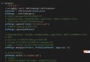
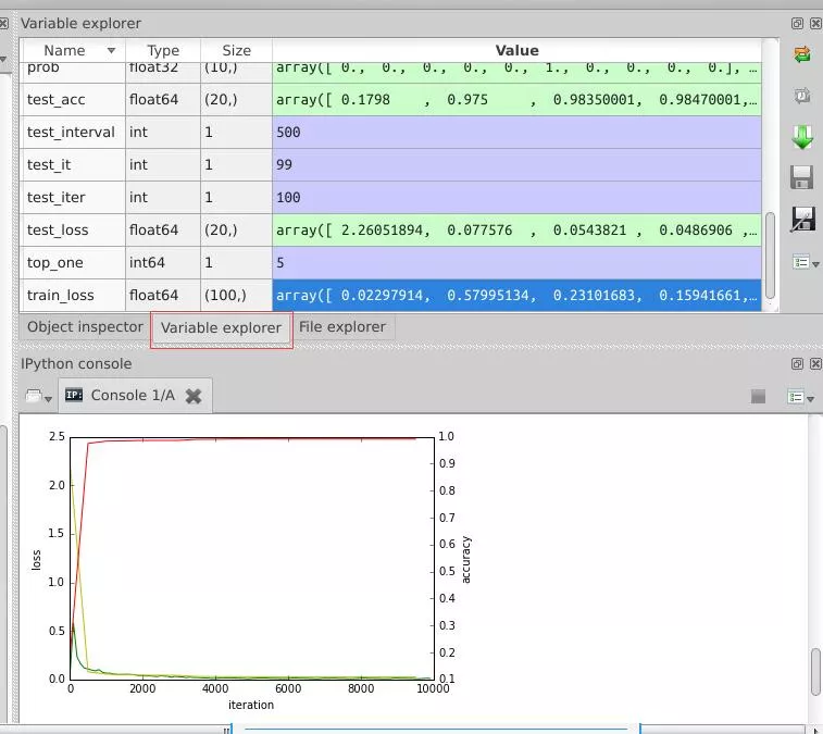
anaconda libraryBecause I use anaconda To install a series of python Third party library , So what I use is spyder, And matlab An editor with a similar interface , At run time , You can view the value of each variable , Easy to understand , Here's the picture :
Once installed anaconda, The operation mode is also very convenient , Input directly at the terminal spyder Just order .
python Interface implementationstay caffe During the training , If we want to know about a certain stage loss Values and accuracy value , And draw it with a chart , use python The interface is right .
# -*- coding: utf-8 -*-"""Created on Tue Jul 19 16:22:22 [email protected]: root"""import matplotlib.pyplot as plt import caffe caffe.set_device(0) caffe.set_mode_gpu() # Use SGDSolver, Random gradient descent algorithm solver = caffe.SGDSolver('/home/xxx/mnist/solver.prototxt') # Equivalent to solver In the document max_iter, That is, the maximum number of solutions niter = 9380 # every other 100 Collect data once at a time display= 100 # Each test is conducted 100 Secondary solution ,10000/100 test_iter = 100 # Every time 500 One test per workout (100 Secondary solution ),60000/64 test_interval =938 # initialization train_loss = zeros(ceil(niter * 1.0 / display)) test_loss = zeros(ceil(niter * 1.0 / test_interval)) test_acc = zeros(ceil(niter * 1.0 / test_interval)) # iteration 0, Not included in solver.step(1) # Auxiliary variable _train_loss = 0; _test_loss = 0; _accuracy = 0 # Do the calculation for it in range(niter): # Perform a solution solver.step(1) # Every iteration , Training batch_size A picture _train_loss += solver.net.blobs['SoftmaxWithLoss1'].data if it % display == 0: # Calculate the average train loss train_loss[it // display] = _train_loss / display _train_loss = 0 if it % test_interval == 0: for test_it in range(test_iter): # Take a test solver.test_nets[0].forward() # Calculation test loss _test_loss += solver.test_nets[0].blobs['SoftmaxWithLoss1'].data # Calculation test accuracy _accuracy += solver.test_nets[0].blobs['Accuracy1'].data # Calculate the average test loss test_loss[it / test_interval] = _test_loss / test_iter # Calculate the average test accuracy test_acc[it / test_interval] = _accuracy / test_iter _test_loss = 0 _accuracy = 0 # draw train loss、test loss and accuracy curve print '\nplot the train loss and test accuracy\n' _, ax1 = plt.subplots() ax2 = ax1.twinx() # train loss -> green ax1.plot(display * arange(len(train_loss)), train_loss, 'g') # test loss -> yellow ax1.plot(test_interval * arange(len(test_loss)), test_loss, 'y') # test accuracy -> Red ax2.plot(test_interval * arange(len(test_acc)), test_acc, 'r') ax1.set_xlabel('iteration') ax1.set_ylabel('loss') ax2.set_ylabel('accuracy') plt.show()The resulting graph is shown in the figure above .
That's all caffe Of python Interface drawing loss and accuracy Details of the curve , More about caffe python draw loss accuracy Please pay attention to other relevant articles of software development network !