This paper introduces a feature selection artifact : Feature selector is a tool for reducing the dimension of machine learning data set , Feature selection can be done foolishly , Just two lines of code !!
source :Will Koehrsen
Code sorting and annotation translation : Huang haiguang
Code and data download address :
github.com/fengdu78/Da…
The selector is based on Python To write , There are five ways to identify features to be deleted :
Feature selector (Feature Selector) Usage of
In this Jupyter In file , We will use FeatureSelector Class to select features to delete from the dataset , This class provides five methods to find the function to be deleted :
FeatureSelector Still under further development ! Welcome to github Submit PR.
from feature_selector import FeatureSelector
import pandas as pd
This data set is used as Kaggle On the housing credit default risk competition (www.kaggle.com/c/home-cred…) Part of the ( Download at the end of the article ). It is designed for supervised machine learning classification tasks , The purpose is to predict whether the customer will default on the loan . You can download the entire dataset here , We will deal with 10,000 A small sample of the row .
Feature selectors are designed for machine learning tasks , But it can be applied to any data set . The method based on feature importance needs to use the supervised learning problem of machine learning .
train = pd.read_csv('data/credit_example.csv')
train_labels = train['TARGET']
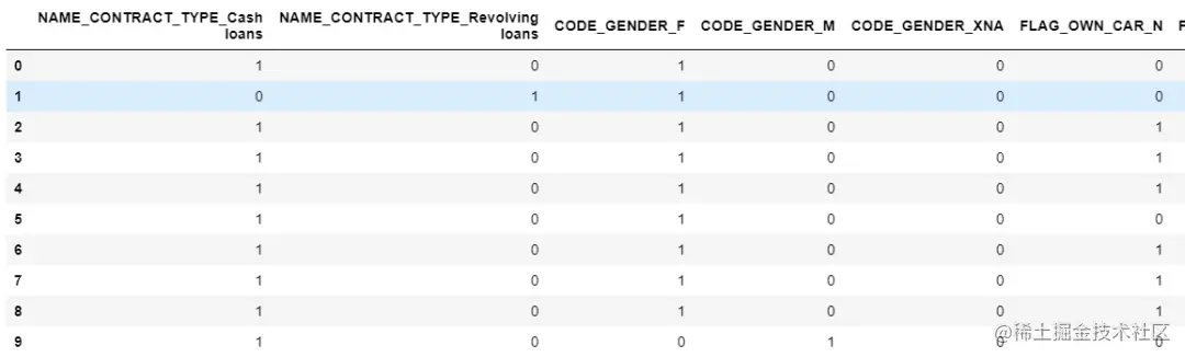
train.head()
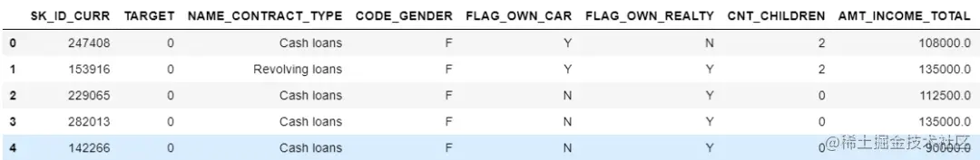
5 rows × 122 columns
There are several classification columns in the dataset .`FeatureSelector` When dealing with the importance of these features, use the unique heat coding .
train = train.drop(columns = ['TARGET'])
stay FeatureSelector Has a for identifying columns , To remove five characteristics :
identify_missing( Find missing values )identify_single_unique( Find a unique value )identify_collinear( Find collinear features )identify_zero_importance ( Find zero important features )identify_low_importance( Find low importance features ) These methods find the features to be deleted according to the specified conditions . The identified features are stored in FeatureSelector Of ops attribute (Python The dictionary ) in . We can manually delete the recognized features , You can also use FeatureSelector The delete feature function in really deletes the feature .
FeatureSelector You only need a dataset that has observations in rows and characteristics in columns ( Standard structured data ). We are dealing with the classification of machine learning , So we also need training labels .
fs = FeatureSelector(data = train, labels = train_labels)
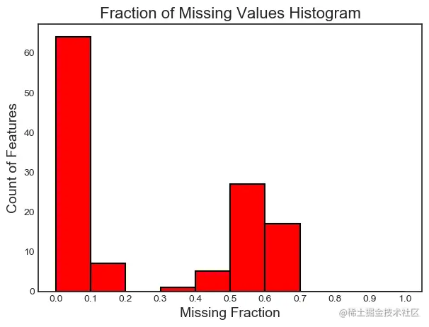
The first feature selection method is simple : Find any columns with missing scores greater than the specified threshold . In this example , We will use the threshold 0.6, This corresponds to finding missing values greater than 60% Characteristics of .( This method does not first encode the feature once ).
fs.identify_missing(missing_threshold=0.6)
17 features with greater than 0.60 missing values.
Can pass FeatureSelector Object's ops Dictionary access has determined the feature to delete .
missing_features = fs.ops['missing']
missing_features[:10]
['OWN_CAR_AGE',
'YEARS_BUILD_AVG',
'COMMONAREA_AVG',
'FLOORSMIN_AVG',
'LIVINGAPARTMENTS_AVG',
'NONLIVINGAPARTMENTS_AVG',
'YEARS_BUILD_MODE',
'COMMONAREA_MODE',
'FLOORSMIN_MODE',
'LIVINGAPARTMENTS_MODE']
We can also plot histograms of missing column scores for all columns in the dataset .
fs.plot_missing()
More about missing scores , We can visit missing_stats attribute , This is the missing score for all features DataFrame.
fs.missing_stats.head(10)
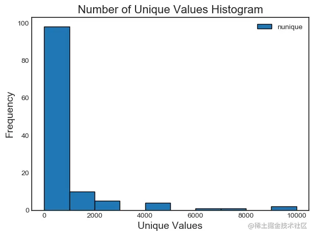
The next method is simple : Find all features that have only one unique value .( This does not uniquely encode features ).
fs.identify_single_unique()
4 features with a single unique value.
single_unique = fs.ops['single_unique']
single_unique
['FLAG_MOBIL', 'FLAG_DOCUMENT_10', 'FLAG_DOCUMENT_12', 'FLAG_DOCUMENT_17']
We can plot a histogram of the number of unique values in each feature in the dataset .
fs.plot_unique()
Last , We can visit a DataFrame, It contains the number of unique values for each feature .
fs.unique_stats.sample(5)
This method finds collinear feature pairs based on Pearson correlation coefficient . For values above the specified threshold ( In absolute terms ) Each pair of , It identifies one of the variables to delete . We need to pass on a correlation_threshold.
This method is based on :chrisalbon.com/machine_lea… Code found in .
For every pair of , The feature to be deleted is in DataFrame The last feature in the column sorting .( Unless one_hot = True, Otherwise, this method will not encode the data once in advance . therefore , Calculate correlation only between numeric columns )
fs.identify_collinear(correlation_threshold=0.975)
24 features with a correlation magnitude greater than 0.97.
correlated_features = fs.ops['collinear']
correlated_features[:5]
['AMT_GOODS_PRICE',
'FLAG_EMP_PHONE',
'YEARS_BUILD_MODE',
'COMMONAREA_MODE',
'ELEVATORS_MODE']
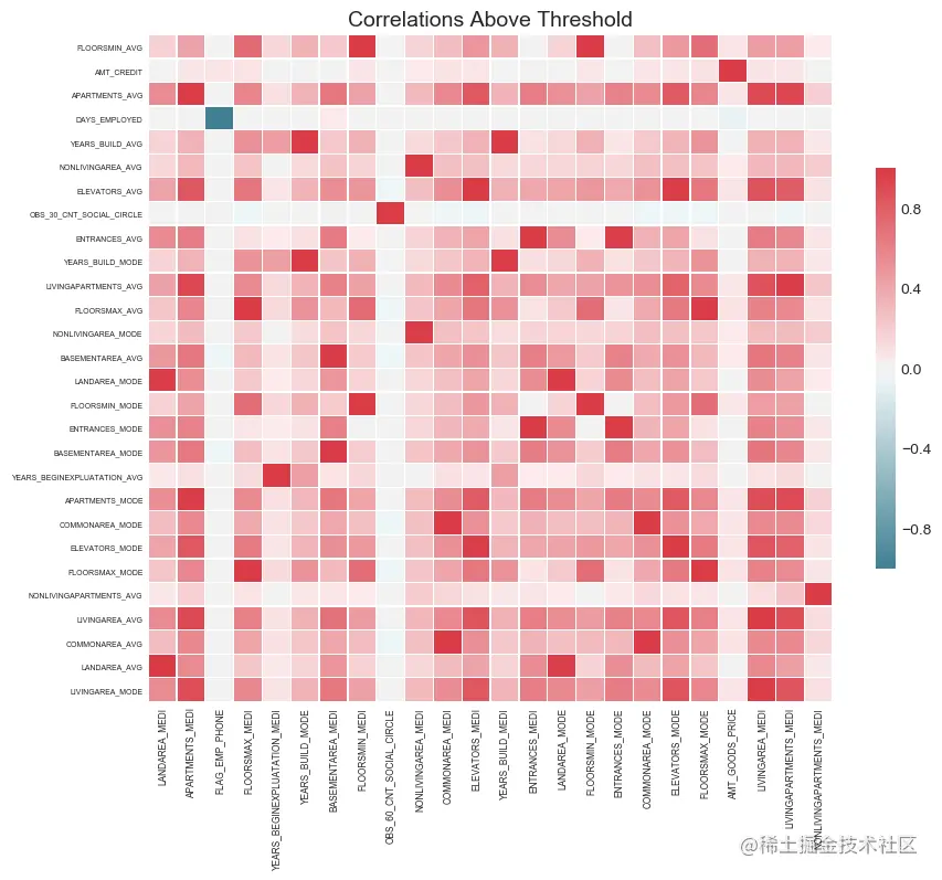
We can see the heat map of the correlation above the threshold . The feature to be deleted is located in x On the shaft .
fs.plot_collinear()
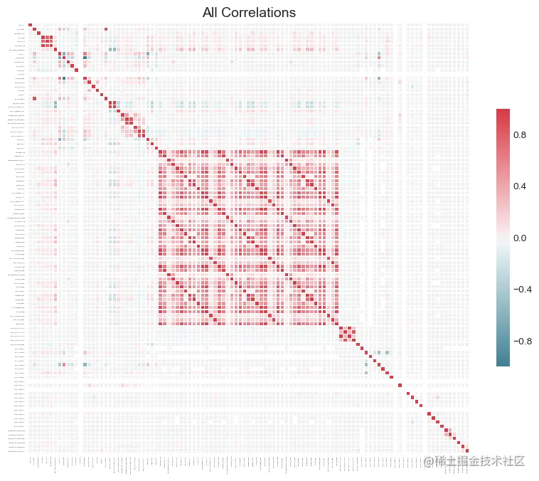
To plot all correlations in the data , We can plot_all = True Pass to plot_collinear function .
fs.plot_collinear(plot_all=True)
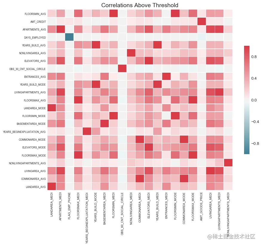
fs.identify_collinear(correlation_threshold=0.98)
fs.plot_collinear()
21 features with a correlation magnitude greater than 0.98.
To view details above the threshold , We visit record_collinear attribute , It's a DataFrame. drop_feature place it on clipboard , And for each feature to be deleted , It is associated with corr_feature There may be multiple correlations , And these correlations are higher than correlation_threshold.
fs.record_collinear.head()
4. Zero important characteristics
This method relies on the machine learning model to identify the features to be deleted . therefore , It is a labeled supervised learning problem . This method uses LightGBM The gradient enhancer implemented in the library finds the importance of features .
In order to reduce the difference of the calculated feature importance , The model is modified by default 10 Time training . By default , Validation sets are also used ( Training data 15%) By stopping the training model in advance , To identify the optimal estimator to be trained . You can pass the following parameters to identify_zero_importance Method :
task: It can be classification or regression. Metrics and tags must match the task .eval_metric: Metrics for early stop ( for example , For classification auc Or for regression l2 ). To view a list of available metrics , see also LightGBM file :(testlightgbm.readthedocs.io/en/latest/P…n_iterations: Training times . The characteristic importance is obtained by averaging in the training operation ( The default is 10).early_stopping: Whether to use early stop when training the model ( Default = True). When the performance of the verification set is for a specified number of estimators ( The default in this implementation is 100) No longer lower , Stopping early will stop training the estimator ( Decision tree ). Early stop is a form of regularization , Used to prevent training data from over fitting . First of all, the data is encoded by single heat , For model use . This means that some zero importance features can be created by one key coding . To view a single encoded column , We can visit FeatureSelector Of one_hot_features .
Be careful : Compared with other methods , The characteristic importance of the model is uncertain ( With a little randomness ). Every time you run this method , The results can change .
fs.identify_zero_importance(task = 'classification', eval_metric = 'auc',
n_iterations = 10, early_stopping = True)
Training Gradient Boosting Model
Training until validation scores don't improve for 100 rounds. Early stopping, best iteration is: [57] valid_0's auc: 0.760957 valid_0's binary_logloss: 0.250579 Training until validation scores don't improve for 100 rounds.
Early stopping, best iteration is:
[29] valid_0's auc: 0.681283 valid_0's binary_logloss: 0.266277
Training until validation scores don't improve for 100 rounds. Early stopping, best iteration is: [50] valid_0's auc: 0.73881 valid_0's binary_logloss: 0.257822 Training until validation scores don't improve for 100 rounds.
Early stopping, best iteration is:
[34] valid_0's auc: 0.720575 valid_0's binary_logloss: 0.262094
Training until validation scores don't improve for 100 rounds. Early stopping, best iteration is: [48] valid_0's auc: 0.769376 valid_0's binary_logloss: 0.247709 Training until validation scores don't improve for 100 rounds.
Early stopping, best iteration is:
[35] valid_0's auc: 0.713877 valid_0's binary_logloss: 0.262254
Training until validation scores don't improve for 100 rounds. Early stopping, best iteration is: [76] valid_0's auc: 0.753081 valid_0's binary_logloss: 0.251867 Training until validation scores don't improve for 100 rounds.
Early stopping, best iteration is:
[70] valid_0's auc: 0.722385 valid_0's binary_logloss: 0.259535
Training until validation scores don't improve for 100 rounds. Early stopping, best iteration is: [45] valid_0's auc: 0.752703 valid_0's binary_logloss: 0.252175 Training until validation scores don't improve for 100 rounds.
Early stopping, best iteration is:
[49] valid_0's auc: 0.757385 valid_0's binary_logloss: 0.250356
81 features with zero importance after one-hot encoding.
To run the gradient lifting model, the features need to be uniquely encoded . These features are preserved in FeatureSelector Of one_hot_features Properties of the . The original features are stored in base_features in .
one_hot_features = fs.one_hot_features
base_features = fs.base_features
print('There are %d original features' % len(base_features))
print('There are %d one-hot features' % len(one_hot_features))
There are 121 original features
There are 134 one-hot features
FeatureSelector Of data Property to save the original DataFrame. After hot coding alone , data_all The attribute will retain the original data as well as the unique hot coded features .
fs.data_all.head(10)
10 rows × 255 columns
We can use a variety of methods to check the results of feature importance . First , We can access a list of features with zero importance .
zero_importance_features = fs.ops['zero_importance']
zero_importance_features[10:15]
['ORGANIZATION_TYPE_Transport: type 1',
'ORGANIZATION_TYPE_Security',
'FLAG_DOCUMENT_15',
'FLAG_DOCUMENT_17',
'ORGANIZATION_TYPE_Religion']
Use plot_feature_importances The feature importance diagram will show us plot_n The most important feature ( The features are summed up as 1). It also shows us the relationship between the cumulative feature importance and the number of features .
When we draw the importance of features , We can pass a threshold , This threshold identifies the number of features required to achieve the specified cumulative feature importance . for example ,threshold = 0.99 Will tell us the total importance of 99% Number of features required .
fs.plot_feature_importances(threshold = 0.99, plot_n = 12)
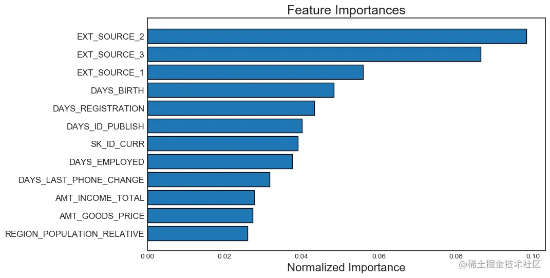
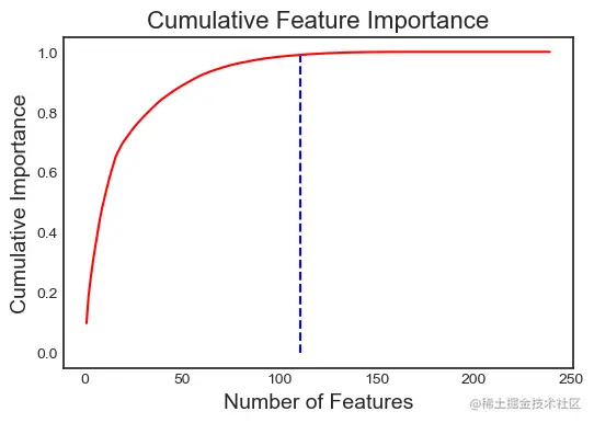
111 features required for 0.99 of cumulative importance
stay FeatureSelector Medium feature_importances Attribute to access all feature importance .
fs.feature_importances.head(10)
We can use these results to select only “ ” One of the most important features . for example , If we want to be in the top 100 Bit is the most important , You can do the following .
one_hundred_features = list(fs.feature_importances.loc[:99, 'feature'])
len(one_hundred_features)
100
This method uses gradient lifting algorithm ( Must first run identify_zero_importance) By finding the feature with the lowest feature importance required to reach the specified cumulative total feature importance , To build feature importance . for example , If we type 0.99, The least important feature importance will be found , These characteristics are less important than the overall characteristics 99%.
When using this method , We must have run identify_zero_importance , And you need to pass a cumulative_importance , This value accounts for a portion of the total characteristic importance .
** Be careful :** This method is based on the importance of gradient lifting model , And it's still uncertain . I recommend running both methods multiple times with different parameters , And test the feature set of each result , Instead of just choosing a number .
fs.identify_low_importance(cumulative_importance = 0.99)
110 features required for cumulative importance of 0.99 after one hot encoding.
129 features do not contribute to cumulative importance of 0.99.
Low importance features to be deleted are those that do not contribute to the specified cumulative importance . These features can also be found in ops Found in the dictionary .
low_importance_features = fs.ops['low_importance']
low_importance_features[:5]
['NAME_FAMILY_STATUS_Widow',
'WEEKDAY_APPR_PROCESS_START_SATURDAY',
'ORGANIZATION_TYPE_Business Entity Type 2',
'ORGANIZATION_TYPE_Business Entity Type 1',
'NAME_INCOME_TYPE_State servant']
Once the feature to be deleted is determined , These features can be deleted in many ways . We can visit removal_ops List of any functions in the dictionary , And manually delete the columns . We can also use remove Method , Pass in the method that identifies the feature we want to delete .
This method returns the result data , Then we can use it for machine learning . It can still be found in the data Property to access the original data .
Note the method used to delete features ! Before using delete feature , It's best to check that you are going to remove Characteristics of .
train_no_missing = fs.remove(methods = ['missing'])
Removed 17 features.
train_no_missing_zero = fs.remove(methods = ['missing', 'zero_importance'])
Removed 98 features.
To delete a feature from all methods , Please pass in method='all'. Before doing this , We can use check_removal Check how many features will be deleted . This will return a list of all features that have been identified for deletion .
all_to_remove = fs.check_removal()
all_to_remove[10:25]
Total of 156 features identified for removal
['FLAG_OWN_REALTY_Y',
'FLAG_DOCUMENT_19',
'ORGANIZATION_TYPE_Agriculture',
'FLOORSMIN_MEDI',
'ORGANIZATION_TYPE_Restaurant',
'NAME_HOUSING_TYPE_With parents',
'NONLIVINGAREA_MEDI',
'NAME_INCOME_TYPE_Pensioner',
'HOUSETYPE_MODE_specific housing',
'ORGANIZATION_TYPE_Industry: type 5',
'ORGANIZATION_TYPE_Realtor',
'OCCUPATION_TYPE_Cleaning staff',
'ORGANIZATION_TYPE_Industry: type 12',
'OCCUPATION_TYPE_Realty agents',
'ORGANIZATION_TYPE_Trade: type 6']
Now we can delete all the recognized features .
train_removed = fs.remove(methods = 'all')
['missing', 'single_unique', 'collinear', 'zero_importance', 'low_importance'] methods have been run
Removed 156 features.
If we look at the returned DataFrame, You may notice several new columns that are not in the original data . These are created when data is uniquely encoded for machine learning . To delete all unique features , We can keep_one_hot = False Pass to remove Method .
train_removed_all = fs.remove(methods = 'all', keep_one_hot=False)
['missing', 'single_unique', 'collinear', 'zero_importance', 'low_importance'] methods have been run
Removed 190 features including one-hot features.
print('Original Number of Features', train.shape[1])
print('Final Number of Features: ', train_removed_all.shape[1])
Original Number of Features 121
Final Number of Features: 65
If we don't want to run one recognition method at a time , You can use identify_all Run all methods in one call . For this function , We need to pass in a parameter dictionary for each individual recognition method .
The following code completes the above steps in one call .
fs = FeatureSelector(data = train, labels = train_labels)
fs.identify_all(selection_params = {'missing_threshold': 0.6, 'correlation_threshold': 0.98,
'task': 'classification', 'eval_metric': 'auc',
'cumulative_importance': 0.99})
17 features with greater than 0.60 missing values.
4 features with a single unique value.
21 features with a correlation magnitude greater than 0.98.
Training Gradient Boosting Model
Training until validation scores don't improve for 100 rounds. Early stopping, best iteration is: [46] valid_0's auc: 0.743917 valid_0's binary_logloss: 0.254668 Training until validation scores don't improve for 100 rounds.
Early stopping, best iteration is:
[82] valid_0's auc: 0.766619 valid_0's binary_logloss: 0.244264
Training until validation scores don't improve for 100 rounds. Early stopping, best iteration is: [55] valid_0's auc: 0.72614 valid_0's binary_logloss: 0.26157 Training until validation scores don't improve for 100 rounds.
Early stopping, best iteration is:
[81] valid_0's auc: 0.756286 valid_0's binary_logloss: 0.251242
Training until validation scores don't improve for 100 rounds. Early stopping, best iteration is: [39] valid_0's auc: 0.686351 valid_0's binary_logloss: 0.269367 Training until validation scores don't improve for 100 rounds.
Early stopping, best iteration is:
[41] valid_0's auc: 0.744124 valid_0's binary_logloss: 0.255549
Training until validation scores don't improve for 100 rounds. Early stopping, best iteration is: [90] valid_0's auc: 0.761742 valid_0's binary_logloss: 0.249119 Training until validation scores don't improve for 100 rounds.
Early stopping, best iteration is:
[49] valid_0's auc: 0.751569 valid_0's binary_logloss: 0.254504
Training until validation scores don't improve for 100 rounds. Early stopping, best iteration is: [76] valid_0's auc: 0.726789 valid_0's binary_logloss: 0.257181 Training until validation scores don't improve for 100 rounds.
Early stopping, best iteration is:
[46] valid_0's auc: 0.714889 valid_0's binary_logloss: 0.260482
80 features with zero importance after one-hot encoding.
115 features required for cumulative importance of 0.99 after one hot encoding.
124 features do not contribute to cumulative importance of 0.99.
150 total features out of 255 identified for removal after one-hot encoding.
train_removed_all_once = fs.remove(methods = 'all', keep_one_hot = True)
['missing', 'single_unique', 'collinear', 'zero_importance', 'low_importance'] methods have been run
Removed 150 features.
fs.feature_importances.head()
The importance of the feature has changed , Therefore, the number of features deleted is slightly different . By the missing (missing)、 Single (single_unique) And collinear ( collinear) Determine that the number of features to delete will remain the same , Because they are deterministic , But because of multiple training models , Zero importance ( zero_importance ) And low importance (low_importance ) The number of features may vary .
This notebook demonstrates how to use FeatureSelector Class to delete features from the dataset . There are several important considerations in this implementation :
In multiple runs of the machine learning model , The importance of features will change .
Decide whether to keep additional features created from a single heat code .
Try several different values for different parameters , To determine which parameters are most appropriate for the machine learning task .
For the same parameters , The lack of (missing)、 Single (single_unique) And collinear ( collinear) The output of will remain unchanged .
Feature selection is a key step in machine learning workflow , It may require multiple iterations to optimize .
I appreciate any comments you have on this project 、 Feedback or help .
Code and data download address :
github.com/fengdu78/Da…
WillKoehrsen:github.com/WillKoehrse…