Pythons meshgrid usage and 3D library MPL_ toolkits. Mplot3d and polynomialfeatures polynomial Library Learning

meshgrid

1 import numpy as np

 2 from matplotlib import pyplot as plt

 3 from mpl_toolkits.mplot3d import Axes3D

 4 x = np.array([0,1,2])

 5 y = np.array([0,1])

 6 X,Y = np.meshgrid(x,y)#X,Y Expanded into a matrix ,

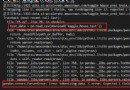
 7 print(X)

 8 print(Y)

 9 theta0, theta1, theta2 = 2, 3, 4

10 ax = Axes3D(plt.figure())# Used to draw three-dimensional drawings

11 Z = theta0 + theta1*X + theta2*Y# seek z value

12 plt.plot(X,Y,'r.')# At this point, you will find that what you draw is 3*2 A little bit , These points form a grid , The coordinates of each tangent point are X*Y Cartesian product of

13 ax.plot_surface(X,Y,Z)# Used to draw three-dimensional drawings

14 plt.show()


1.
2.
3.
4.
5.
6.
7.
8.
9.
10.
11.
12.
13.
14.

​​ You can also refer to this blog for details

mpl_toolkits.mplot3d

​​ About 3D Drawing blog

The method of dividing panels is used in drawing

Use add_subplot

import numpy as np

import matplotlib.pyplot as plt

x = np.arange(0, 100)

fig = plt.figure()

ax1 = fig.add_subplot(221)

ax1.plot(x, x)

ax2 = fig.add_subplot(222)

ax2.plot(x, -x)

ax3 = fig.add_subplot(223)

ax3.plot(x, x ** 2)

ax4 = fig.add_subplot(224)

ax4.plot(x, np.log(x))

plt.show()


1.
2.
3.
4.
5.
6.
7.
8.
9.
10.
11.
12.
13.

Use subplot Method

import numpy as np

from matplotlib import pyplot as plt

x = np.arange(10)

plt.subplot(221)

plt.plot(x,x)

plt.subplot(223)

plt.plot(x,-x)

plt.show()


1.
2.
3.
4.
5.
6.
7.
8.

PolynomialFeatures

1 import numpy as np

 2 import matplotlib.pyplot as plt

 3 from sklearn.preprocessing import PolynomialFeatures# polynomial

 4 from sklearn.linear_model import LinearRegression

 5

 6 # Load data

 7 data = np.genfromtxt("job.csv", delimiter=",")

 8 x_data = data[1:,1]

 9 y_data = data[1:,2]

10 plt.scatter(x_data,y_data)

11 plt.show()

12 # Dimension must be two-dimensional

13 x_data = x_data[:,np.newaxis]

14 y_data = y_data[:,np.newaxis]

15 # Define polynomial regression ,degree The value of can adjust the characteristic of the polynomial

16 poly = PolynomialFeatures(degree=4)

17 # Feature handling

18 x_poly = poly.fit_transform(x_data)

19 # Define the regression model

20 model = LinearRegression()

21 # Training models

22 model.fit(x_poly,y_data)

23 plt.plot(x_data,y_data,'b.')

24 plt.plot(x_data,model.predict(poly.fit_transform(x_data)),'r')

25 plt.show()


1.
2.
3.
4.
5.
6.
7.
8.
9.
10.
11.
12.
13.
14.
15.
16.
17.
18.
19.
20.
21.
22.
23.
24.
25.

author ： Your Rego

The copyright of this article belongs to the author , Welcome to reprint , But without the author's consent, the original link must be given on the article page , Otherwise, the right to pursue legal responsibility is reserved .