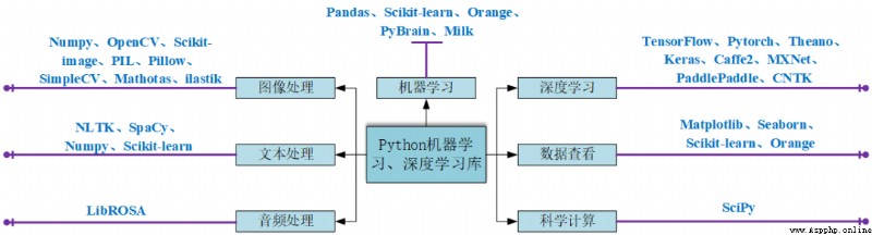
In order that we can understand the commonly used Python Library has a preliminary understanding , Learn by selecting a library that can meet your needs , This paper briefly and comprehensively introduces the common artificial intelligence database at present .
1、Numpy
NumPy(Numerical Python) yes Python An extension library , Support a large number of dimension arrays and matrix operations , In addition, it also provides a large number of mathematical function libraries for array operation ,Numpy Bottom use C Language writing , Storing objects directly in an array , Instead of storing object pointers , Therefore, its computational efficiency is much higher than that of pure Python Code .
We can compare the pure Python And use Numpy Library in calculation list sin Speed comparison of values :
import numpy as np
import math
import random
import time
start = time.time()
for i in range(10):
    list_1 = list(range(1,10000))
    for j in range(len(list_1)):
        list_1[j] = math.sin(list_1[j])
print(" Use pure Python when {}s".format(time.time()-start))
start = time.time()
for i in range(10):
    list_1 = np.array(np.arange(1,10000))
    list_1 = np.sin(list_1)
print(" Use Numpy when {}s".format(time.time()-start))
Run the results from the following , You can see the use of Numpy The library is faster than pure Python Code written :
Use pure Python when 0.017444372177124023s
Use Numpy when 0.001619577407836914s
2、OpenCV
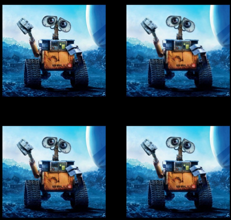
OpenCV Is a cross platform computer vision library , Can run in Linux、Windows and Mac OS On the operating system . It's lightweight and efficient —— By a series of C Functions and small quantities C++ Class a , It also provides Python Interface , Many general algorithms in image processing and computer vision are realized . The following code tries to use some simple filters , Including image smoothing 、 Gauss blur, etc :
import numpy as np
import cv2 as cv
from matplotlib import pyplot as plt
img = cv.imread('h89817032p0.png')
kernel = np.ones((5,5),np.float32)/25
dst = cv.filter2D(img,-1,kernel)
blur_1 = cv.GaussianBlur(img,(5,5),0)
blur_2 = cv.bilateralFilter(img,9,75,75)
plt.figure(figsize=(10,10))
plt.subplot(221),plt.imshow(img[:,:,::-1]),plt.title('Original')
plt.xticks([]), plt.yticks([])
plt.subplot(222),plt.imshow(dst[:,:,::-1]),plt.title('Averaging')
plt.xticks([]), plt.yticks([])
plt.subplot(223),plt.imshow(blur_1[:,:,::-1]),plt.title('Gaussian')
plt.xticks([]), plt.yticks([])
plt.subplot(224),plt.imshow(blur_1[:,:,::-1]),plt.title('Bilateral')
plt.xticks([]), plt.yticks([])
plt.show()
You need a video tutorial. Add the following little sister to get it !
3、Scikit-image
scikit-image Is based on scipy Image processing library , It takes pictures as numpy Array processing .
for example , You can use scikit-image Change the picture scale ,scikit-image Provides rescale、resize as well as downscale_local_mean Such as function .
from skimage import data, color, io
from skimage.transform import rescale, resize, downscale_local_mean
image = color.rgb2gray(io.imread('h89817032p0.png'))
image_rescaled = rescale(image, 0.25, anti_aliasing=False)
image_resized = resize(image, (image.shape[0] // 4, image.shape[1] // 4),
                       anti_aliasing=True)
image_downscaled = downscale_local_mean(image, (4, 3))
plt.figure(figsize=(20,20))
plt.subplot(221),plt.imshow(image, cmap='gray'),plt.title('Original')
plt.xticks([]), plt.yticks([])
plt.subplot(222),plt.imshow(image_rescaled, cmap='gray'),plt.title('Rescaled')
plt.xticks([]), plt.yticks([])
plt.subplot(223),plt.imshow(image_resized, cmap='gray'),plt.title('Resized')
plt.xticks([]), plt.yticks([])
plt.subplot(224),plt.imshow(image_downscaled, cmap='gray'),plt.title('Downscaled')
plt.xticks([]), plt.yticks([])
plt.show()
4、PIL
Python Imaging Library(PIL) Has become a Python In fact, the image processing standard library , This is because ,PIL Very powerful , but API It's very easy to use .
But because of PIL Only to Python 2.7, Plus years of disrepair , So a group of volunteers were PIL A compatible version of , Name is Pillow, Support the latest Python 3.x, Many new features have been added , therefore , We can skip PIL, Direct installation and use Pillow.
5、Pillow
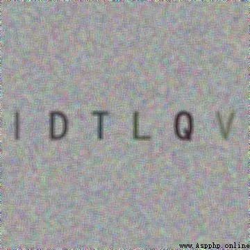
Use Pillow Generate letter verification code picture :
from PIL import Image, ImageDraw, ImageFont, ImageFilter
import random
#  Random letters :
def rndChar():
    return chr(random.randint(65, 90))
#  Random color 1:
def rndColor():
    return (random.randint(64, 255), random.randint(64, 255), random.randint(64, 255))
#  Random color 2:
def rndColor2():
    return (random.randint(32, 127), random.randint(32, 127), random.randint(32, 127))
# 240 x 60:
width = 60 * 6
height = 60 * 6
image = Image.new('RGB', (width, height), (255, 255, 255))
#  establish Font object :
font = ImageFont.truetype('/usr/share/fonts/wps-office/simhei.ttf', 60)
#  establish Draw object :
draw = ImageDraw.Draw(image)
#  Fill each pixel :
for x in range(width):
    for y in range(height):
        draw.point((x, y), fill=rndColor())
#  Output text :
for t in range(6):
    draw.text((60 * t + 10, 150), rndChar(), font=font, fill=rndColor2())
#  Fuzzy :
image = image.filter(ImageFilter.BLUR)
image.save('code.jpg', 'jpeg')
6、SimpleCV
SimpleCV Is an open source framework for building computer vision applications . Use it , Access to high-performance computer vision Libraries , Such as OpenCV, You don't have to know the bit depth first 、 File format 、 Color space 、 Buffer management 、 Terms such as eigenvalues or matrices . But for Python3 Your support is very poor, very poor , stay Python3.7 Use the following code :
from SimpleCV import Image, Color, Display
# load an image from imgur
img = Image('http://i.imgur.com/lfAeZ4n.png')
# use a keypoint detector to find areas of interest
feats = img.findKeypoints()
# draw the list of keypoints
feats.draw(color=Color.RED)
# show the  resulting image.
img.show()
# apply the stuff we found to the image.
output = img.applyLayers()
# save the results.
output.save('juniperfeats.png')
The following errors will be reported , Therefore, it is not recommended to Python3 Use in :
SyntaxError: Missing parentheses in call to 'print'. Did you mean print('unit test')?
7、Mahotas
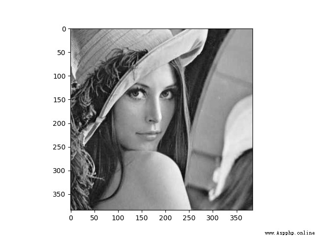
Mahotas Is a fast computer vision algorithm library , It's built on Numpy above , At present, it has more than 100 An image processing and computer vision function , And growing .
Use Mahotas Load image , And operate the pixels :
import numpy as np
import mahotas
import mahotas.demos
from mahotas.thresholding import soft_threshold
from matplotlib import pyplot as plt
from os import path
f = mahotas.demos.load('lena', as_grey=True)
f = f[128:,128:]
plt.gray()
# Show the data:
print("Fraction of zeros in original image: {0}".format(np.mean(f==0)))
plt.imshow(f)
plt.show()
8、Ilastik
Ilastik It can provide users with good biological information image analysis services based on machine learning , Using machine learning algorithms , Easily split , classification , Track and count cells or other experimental data . Most operations are interactive , There is no need for machine learning expertise .
9、Scikit-learn
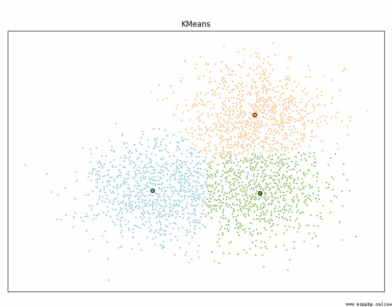
Scikit-learn Is aimed at Python Free software machine learning library for programming languages . It has various classifications , Regression and clustering algorithms , Including support vector machines , Random forests , Gradient rise ,k Mean and DBSCAN And many other machine learning algorithms .
Use Scikit-learn Realization KMeans Algorithm :
import time
import numpy as np
import matplotlib.pyplot as plt
from sklearn.cluster import MiniBatchKMeans, KMeans
from sklearn.metrics.pairwise import pairwise_distances_argmin
from sklearn.datasets import make_blobs
# Generate sample data
np.random.seed(0)
batch_size = 45
centers = [[1, 1], [-1, -1], [1, -1]]
n_clusters = len(centers)
X, labels_true = make_blobs(n_samples=3000, centers=centers, cluster_std=0.7)
# Compute clustering with Means
k_means = KMeans(init='k-means++', n_clusters=3, n_init=10)
t0 = time.time()
k_means.fit(X)
t_batch = time.time() - t0
# Compute clustering with MiniBatchKMeans
mbk = MiniBatchKMeans(init='k-means++', n_clusters=3, batch_size=batch_size,
                      n_init=10, max_no_improvement=10, verbose=0)
t0 = time.time()
mbk.fit(X)
t_mini_batch = time.time() - t0
# Plot result
fig = plt.figure(figsize=(8, 3))
fig.subplots_adjust(left=0.02, right=0.98, bottom=0.05, top=0.9)
colors = ['#4EACC5', '#FF9C34', '#4E9A06']
# We want to have the same colors for the same cluster from the
# MiniBatchKMeans and the KMeans algorithm. Let's pair the cluster centers per
# closest one.
k_means_cluster_centers = k_means.cluster_centers_
order = pairwise_distances_argmin(k_means.cluster_centers_,
                                  mbk.cluster_centers_)
mbk_means_cluster_centers = mbk.cluster_centers_[order]
k_means_labels = pairwise_distances_argmin(X, k_means_cluster_centers)
mbk_means_labels = pairwise_distances_argmin(X, mbk_means_cluster_centers)
# KMeans
for k, col in zip(range(n_clusters), colors):
    my_members = k_means_labels == k
    cluster_center = k_means_cluster_centers[k]
    plt.plot(X[my_members, 0], X[my_members, 1], 'w',
            markerfacecolor=col, marker='.')
    plt.plot(cluster_center[0], cluster_center[1], 'o', markerfacecolor=col,
            markeredgecolor='k', markersize=6)
plt.title('KMeans')
plt.xticks(())
plt.yticks(())
plt.show()
10、SciPy
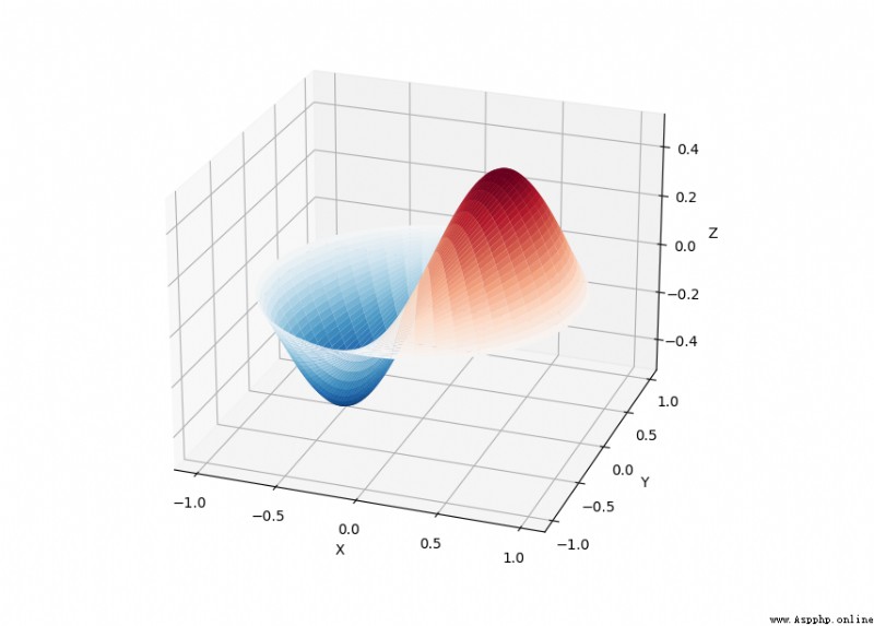
SciPy The library provides many user-friendly and efficient numerical calculations , Such as numerical integration 、 interpolation 、 Optimize 、 Linear algebra, etc .
SciPy The library defines many special functions in Mathematical Physics , Including elliptic functions 、 Bessel function 、 Gamma function 、 Beta function 、 Hypergeometric functions 、 Parabolic cylindrical function, etc .
from scipy import special
import matplotlib.pyplot as plt
import numpy as np
def drumhead_height(n, k, distance, angle, t):
    kth_zero = special.jn_zeros(n, k)[-1]
    return np.cos(t) * np.cos(n*angle) * special.jn(n, distance*kth_zero)
theta = np.r_[0:2*np.pi:50j]
radius = np.r_[0:1:50j]
x = np.array([r * np.cos(theta) for r in radius])
y = np.array([r * np.sin(theta) for r in radius])
z = np.array([drumhead_height(1, 1, r, theta, 0.5) for r in radius])
fig = plt.figure()
ax = fig.add_axes(rect=(0, 0.05, 0.95, 0.95), projection='3d')
ax.plot_surface(x, y, z, rstride=1, cstride=1, cmap='RdBu_r', vmin=-0.5, vmax=0.5)
ax.set_xlabel('X')
ax.set_ylabel('Y')
ax.set_xticks(np.arange(-1, 1.1, 0.5))
ax.set_yticks(np.arange(-1, 1.1, 0.5))
ax.set_zlabel('Z')
plt.show()
11、NLTK
NLTK Is build Python A library of programs to deal with natural languages . It's for 50 Multiple corpora and vocabulary resources ( Such as WordNet ) Provides an easy to use interface , And a set for classification 、 participle 、 Word stem 、 Mark 、 Text processing library for parsing and semantic reasoning 、 Industrial natural language processing (Natural Language Processing, NLP) The wrapper for the library .
NLTK go by the name of “a wonderful tool for teaching, and working in, computational linguistics using Python”.
import nltk
from nltk.corpus import treebank
#  You need to download it for the first time
nltk.download('punkt')
nltk.download('averaged_perceptron_tagger')
nltk.download('maxent_ne_chunker')
nltk.download('words')
nltk.download('treebank')
sentence = """At eight o'clock on Thursday morning Arthur didn't feel very good."""
# Tokenize
tokens = nltk.word_tokenize(sentence)
tagged = nltk.pos_tag(tokens)
# Identify named entities
entities = nltk.chunk.ne_chunk(tagged)
# Display a parse tree
t = treebank.parsed_sents('wsj_0001.mrg')[0]
t.draw()

12、spaCy
spaCy It's a free open source library , be used for Python Advanced in NLP. It can be used to build applications that handle large amounts of text ; It can also be used to build information extraction or natural language understanding systems , Or preprocess the text for deep learning .
  import spacy
  texts = [
      "Net income was $9.4 million compared to the prior year of $2.7 million.",
      "Revenue exceeded twelve billion dollars, with a loss of $1b.",
  ]
  nlp = spacy.load("en_core_web_sm")
  for doc in nlp.pipe(texts, disable=["tok2vec", "tagger", "parser", "attribute_ruler", "lemmatizer"]):
      # Do something with the doc here
      print([(ent.text, ent.label_) for ent in doc.ents])
nlp.pipe Generate Doc object , So we can iterate over them and access the named entity prediction :
[('$9.4 million', 'MONEY'), ('the prior year', 'DATE'), ('$2.7 million', 'MONEY')]
[('twelve billion dollars', 'MONEY'), ('1b', 'MONEY')]
You need a video tutorial. Add the following little sister to get it !
13、LibROSA
librosa Is a for music and audio analysis Python library , It provides the functions and functions necessary to create a music information retrieval system .
# Beat tracking example
import librosa
# 1. Get the file path to an included audio example
filename = librosa.example('nutcracker')
# 2. Load the audio as a waveform `y`
#    Store the sampling rate as `sr`
y, sr = librosa.load(filename)
# 3. Run the default beat tracker
tempo, beat_frames = librosa.beat.beat_track(y=y, sr=sr)
print('Estimated tempo: {:.2f} beats per minute'.format(tempo))
# 4. Convert the frame indices of beat events into timestamps
beat_times = librosa.frames_to_time(beat_frames, sr=sr)
14、Pandas
Pandas It's a fast one 、 Powerful 、 Flexible and easy to use open source data analysis and operation tools , Pandas From various file formats, such as CSV、JSON、SQL、Microsoft Excel Import data , It can operate on various data , Like merging 、 Reshaping 、 choice , There are also data cleaning and data processing features .Pandas Widely used in academic 、 Finance 、 Statistics and other data analysis fields .
import matplotlib.pyplot as plt
import pandas as pd
import numpy as np
ts = pd.Series(np.random.randn(1000), index=pd.date_range("1/1/2000", periods=1000))
ts = ts.cumsum()
df = pd.DataFrame(np.random.randn(1000, 4), index=ts.index, columns=list("ABCD"))
df = df.cumsum()
df.plot()
plt.show()
15、Matplotlib
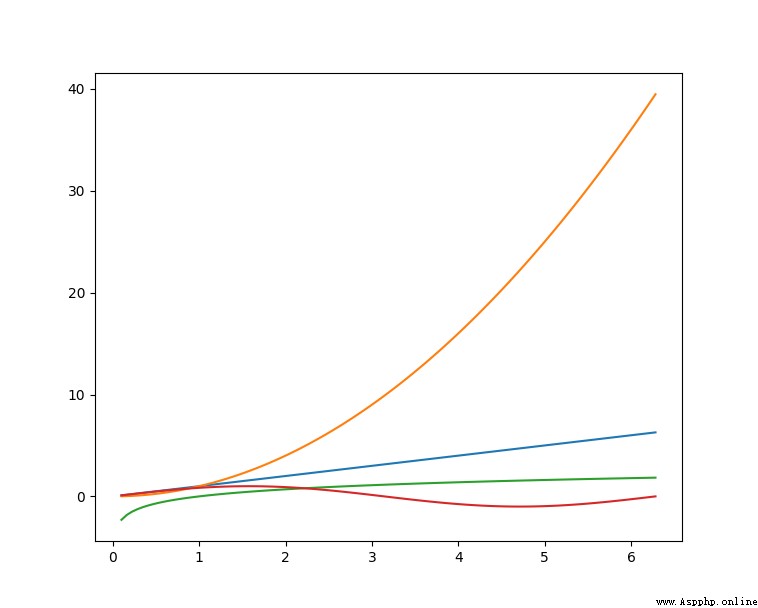
Matplotlib yes Python Drawing library of , It offers a complete set and matlab Similar orders API, It can generate exquisite graphics of publishing quality level ,Matplotlib Make drawing very simple , Excellent balance between ease of use and performance .
Use Matplotlib Draw a multi curve :
# plot_multi_curve.py
import numpy as np
import matplotlib.pyplot as plt
x = np.linspace(0.1, 2 * np.pi, 100)
y_1 = x
y_2 = np.square(x)
y_3 = np.log(x)
y_4 = np.sin(x)
plt.plot(x,y_1)
plt.plot(x,y_2)
plt.plot(x,y_3)
plt.plot(x,y_4)
plt.show()
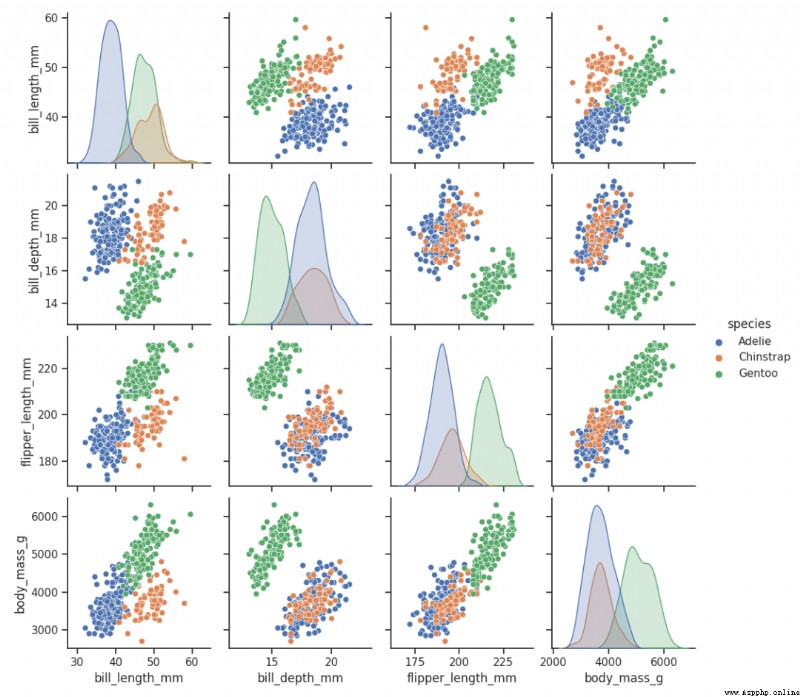
16、Seaborn
Seaborn Is in Matplotlib On the basis of a more advanced API Packaged Python Data visualization Library , So it's easier to draw , Should put the Seaborn As Matplotlib A supplement to , It's not a substitute .
import seaborn as sns
import matplotlib.pyplot as plt
sns.set_theme()
df = sns.load_dataset("penguins")
sns.pairplot(df, hue="species")
plt.show()
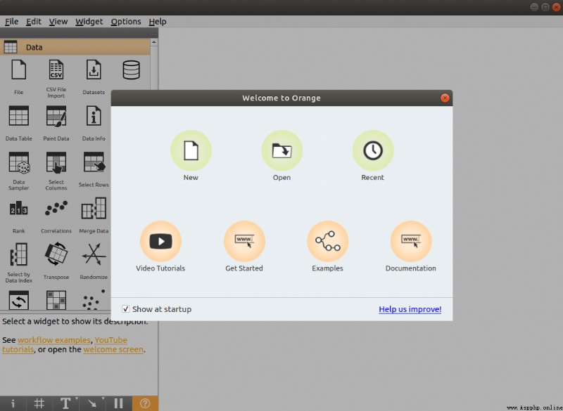
17、Orange
Orange Is an open source data mining and machine learning software , Provides a series of data exploration 、 visualization 、 Preprocessing and modeling components .Orange Beautiful and intuitive interactive user interface , It is very suitable for novices to carry out exploratory data analysis and visual display ; At the same time, advanced users can also use it as Python A programming module for data operation and component development .
Use pip You can install Orange, Praise ~
$ pip install orange3
After installation , Enter at the command line orange-canvas Command to start Orange The graphical interface :
$ orange-canvas
After startup , You can see Orange The graphical interface , All kinds of operations .
18、PyBrain
PyBrain yes Python Modular machine learning library . Its goal is to provide flexibility for machine learning tasks and various predefined environments 、 Easy to use and powerful algorithms to test and compare algorithms .PyBrain yes Python-Based Reinforcement Learning, Artificial Intelligence and Neural Network Library Abbreviation .
We will use a simple example to show PyBrain Usage of , Build a multi-layer perceptron (Multi Layer Perceptron, MLP).
First , We create a new feedforward network object :
from pybrain.structure import FeedForwardNetwork
n = FeedForwardNetwork()
Next , Build input 、 Hide and output layers :
from pybrain.structure import LinearLayer, SigmoidLayer
inLayer = LinearLayer(2)
hiddenLayer = SigmoidLayer(3)
outLayer = LinearLayer(1)
In order to use the constructed layer , They must be added to the network :
n.addInputModule(inLayer)
n.addModule(hiddenLayer)
n.addOutputModule(outLayer)
Multiple input and output modules can be added . For forward calculation and back error propagation , The network must know which layers are input 、 Which layers are output .
This requires a clear determination of how they should be connected . So , We use the most common connection type , Fully connected layer , from FullConnection Class implementation :
from pybrain.structure import FullConnection
in_to_hidden = FullConnection(inLayer, hiddenLayer)
hidden_to_out = FullConnection(hiddenLayer, outLayer)
Same as layer , We must explicitly add them to the network :
n.addConnection(in_to_hidden)
n.addConnection(hidden_to_out)
All elements are now in place , Last , We need to call .sortModules() Method makes MLP You can use :
n.sortModules()
This call performs some internal initialization , This is necessary before using the network .
19、Milk
MILK(MACHINE LEARNING TOOLKIT) yes Python Machine learning toolkit for language . It mainly contains many classifiers, such as SVMS、K-NN、 Supervised classification is used in random forest and decision tree , It can also perform feature selection , Different forms can be formed, such as unsupervised learning 、 Close relationship spread and by MILK Supported by K-means Clustering and other classification systems .
Use MILK Training a classifier :
import numpy as np
import milk
features = np.random.rand(100,10)
labels = np.zeros(100)
features[50:] += .5
labels[50:] = 1
learner = milk.defaultclassifier()
model = learner.train(features, labels)
# Now you can use the model on new examples:
example = np.random.rand(10)
print(model.apply(example))
example2 = np.random.rand(10)
example2 += .5
print(model.apply(example2))
20、TensorFlow
TensorFlow It is an end-to-end open source machine learning platform . It has a comprehensive and flexible ecosystem , Generally, it can be divided into TensorFlow1.x and TensorFlow2.x,TensorFlow1.x And TensorFlow2.x The main difference is TF1.x Use static diagrams instead of TF2.x Use Eager Mode Dynamic graph .
It's mainly used here TensorFlow2.x As an example , On display in TensorFlow2.x Constructing convolutional neural network (Convolutional Neural Network, CNN).
import tensorflow as tf
from tensorflow.keras import datasets, layers, models
#  Data loading
(train_images, train_labels), (test_images, test_labels) = datasets.cifar10.load_data()
#  Data preprocessing
train_images, test_images = train_images / 255.0, test_images / 255.0
#  model building
model = models.Sequential()
model.add(layers.Conv2D(32, (3, 3), activation='relu', input_shape=(32, 32, 3)))
model.add(layers.MaxPooling2D((2, 2)))
model.add(layers.Conv2D(64, (3, 3), activation='relu'))
model.add(layers.MaxPooling2D((2, 2)))
model.add(layers.Conv2D(64, (3, 3), activation='relu'))
model.add(layers.Flatten())
model.add(layers.Dense(64, activation='relu'))
model.add(layers.Dense(10))
#  Model compilation and training
model.compile(optimizer='adam',
              loss=tf.keras.losses.SparseCategoricalCrossentropy(from_logits=True),
              metrics=['accuracy'])
history = model.fit(train_images, train_labels, epochs=10,
                    validation_data=(test_images, test_labels))
You need a video tutorial. Add the following little sister to get it !
21、PyTorch
PyTorch The predecessor was Torch, Its bottom layer and Torch Frame like , But use Python A lot of things have been rewritten , Not only more flexible , Support dynamic graph , And it provides Python Interface .
#  Import library
import torch
from torch import nn
from torch.utils.data import DataLoader
from torchvision import datasets
from torchvision.transforms import ToTensor, Lambda, Compose
import matplotlib.pyplot as plt
#  model building
device = "cuda" if torch.cuda.is_available() else "cpu"
print("Using {} device".format(device))
# Define model
class NeuralNetwork(nn.Module):
    def __init__(self):
        super(NeuralNetwork, self).__init__()
        self.flatten = nn.Flatten()
        self.linear_relu_stack = nn.Sequential(
            nn.Linear(28*28, 512),
            nn.ReLU(),
            nn.Linear(512, 512),
            nn.ReLU(),
            nn.Linear(512, 10),
            nn.ReLU()
        )
    def forward(self, x):
        x = self.flatten(x)
        logits = self.linear_relu_stack(x)
        return logits
model = NeuralNetwork().to(device)
#  Loss function and optimizer
loss_fn = nn.CrossEntropyLoss()
optimizer = torch.optim.SGD(model.parameters(), lr=1e-3)
#  model training
def train(dataloader, model, loss_fn, optimizer):
    size = len(dataloader.dataset)
    for batch, (X, y) in enumerate(dataloader):
        X, y = X.to(device), y.to(device)
        # Compute prediction error
        pred = model(X)
        loss = loss_fn(pred, y)
        # Backpropagation
        optimizer.zero_grad()
        loss.backward()
        optimizer.step()
        if batch % 100 == 0:
            loss, current = loss.item(), batch * len(X)
            print(f"loss: {loss:>7f}  [{current:>5d}/{size:>5d}]")
22、Theano
Theano It's a Python library , It allows you to define 、 Optimize and efficiently compute mathematical expressions involving multidimensional arrays , Built on NumPy above .
stay Theano Calculation of Jacobian matrix :
import theano
import theano.tensor as T
x = T.dvector('x')
y = x ** 2
J, updates = theano.scan(lambda i, y,x : T.grad(y[i], x), sequences=T.arange(y.shape[0]), non_sequences=[y,x])
f = theano.function([x], J, updates=updates)
f([4, 4])
23、Keras
Keras It's a use. Python Advanced neural network API, It can take TensorFlow, CNTK, perhaps Theano Run as back end .Keras The focus of development is to support rapid experiments , Be able to convert ideas into experimental results with minimal delay .
from keras.models import Sequential
from keras.layers import Dense
#  model building
model = Sequential()
model.add(Dense(units=64, activation='relu', input_dim=100))
model.add(Dense(units=10, activation='softmax'))
#  Model compilation and training
model.compile(loss='categorical_crossentropy',
              optimizer='sgd',
              metrics=['accuracy'])
model.fit(x_train, y_train, epochs=5, batch_size=32)
24、Caffe
stay Caffe2 On the official website , So to speak :Caffe2 Now it is PyTorch Part of . Although these api Will continue to work , But encourage the use of PyTorch api.
25、MXNet
MXNet It is a deep learning framework designed for efficiency and flexibility . It allows mixed symbolic programming and imperative programming , To maximize efficiency and productivity . Use MXNet Build handwritten numeral recognition model :
import mxnet as mx
from mxnet import gluon
from mxnet.gluon import nn
from mxnet import autograd as ag
import mxnet.ndarray as F
#  Data loading
mnist = mx.test_utils.get_mnist()
batch_size = 100
train_data = mx.io.NDArrayIter(mnist['train_data'], mnist['train_label'], batch_size, shuffle=True)
val_data = mx.io.NDArrayIter(mnist['test_data'], mnist['test_label'], batch_size)
# CNN Model
class Net(gluon.Block):
    def __init__(self, **kwargs):
        super(Net, self).__init__(**kwargs)
        self.conv1 = nn.Conv2D(20, kernel_size=(5,5))
        self.pool1 = nn.MaxPool2D(pool_size=(2,2), strides = (2,2))
        self.conv2 = nn.Conv2D(50, kernel_size=(5,5))
        self.pool2 = nn.MaxPool2D(pool_size=(2,2), strides = (2,2))
        self.fc1 = nn.Dense(500)
        self.fc2 = nn.Dense(10)
    def forward(self, x):
        x = self.pool1(F.tanh(self.conv1(x)))
        x = self.pool2(F.tanh(self.conv2(x)))
        # 0 means copy over size from corresponding dimension.
        # -1 means infer size from the rest of dimensions.
        x = x.reshape((0, -1))
        x = F.tanh(self.fc1(x))
        x = F.tanh(self.fc2(x))
        return x
net = Net()
#  Initialization and optimizer definition
# set the context on GPU is available otherwise CPU
ctx = [mx.gpu() if mx.test_utils.list_gpus() else mx.cpu()]
net.initialize(mx.init.Xavier(magnitude=2.24), ctx=ctx)
trainer = gluon.Trainer(net.collect_params(), 'sgd', {'learning_rate': 0.03})
#  model training
# Use Accuracy as the evaluation metric.
metric = mx.metric.Accuracy()
softmax_cross_entropy_loss = gluon.loss.SoftmaxCrossEntropyLoss()
for i in range(epoch):
    # Reset the train data iterator.
    train_data.reset()
    for batch in train_data:
        data = gluon.utils.split_and_load(batch.data[0], ctx_list=ctx, batch_axis=0)
        label = gluon.utils.split_and_load(batch.label[0], ctx_list=ctx, batch_axis=0)
        outputs = []
        # Inside training scope
        with ag.record():
            for x, y in zip(data, label):
                z = net(x)
                # Computes softmax cross entropy loss.
                loss = softmax_cross_entropy_loss(z, y)
                # Backpropogate the error for one iteration.
                loss.backward()
                outputs.append(z)
        metric.update(label, outputs)
        trainer.step(batch.data[0].shape[0])
    # Gets the evaluation result.
    name, acc = metric.get()
    # Reset evaluation result to initial state.
    metric.reset()
    print('training acc at epoch %d: %s=%f'%(i, name, acc))
26、PaddlePaddle
Flying propeller (PaddlePaddle) Based on Baidu's years of deep learning technology research and business application , Set deep learning core training and reasoning framework 、 Basic model base 、 End to end Development Suite 、 Rich tool components in one . It is the first independent R & D project in China 、 Fully functional 、 Open source and open industrial deep learning platform .
Use PaddlePaddle Realization LeNtet5:
#  Import required packages
import paddle
import numpy as np
from paddle.nn import Conv2D, MaxPool2D, Linear
##  networking
import paddle.nn.functional as F
#  Definition  LeNet  Network structure
class LeNet(paddle.nn.Layer):
    def __init__(self, num_classes=1):
        super(LeNet, self).__init__()
        #  Create convolution and pooling layers
        #  Create the 1 Convolution layers
        self.conv1 = Conv2D(in_channels=1, out_channels=6, kernel_size=5)
        self.max_pool1 = MaxPool2D(kernel_size=2, stride=2)
        #  The logic of size : The number of channels is not changed in the pool layer ; The current number of channels is 6
        #  Create the 2 Convolution layers
        self.conv2 = Conv2D(in_channels=6, out_channels=16, kernel_size=5)
        self.max_pool2 = MaxPool2D(kernel_size=2, stride=2)
        #  Create the 3 Convolution layers
        self.conv3 = Conv2D(in_channels=16, out_channels=120, kernel_size=4)
        #  The logic of size : The input layer flattens the data [B,C,H,W] -> [B,C*H*W]
        #  Input size yes [28,28], After three convolutions and two pooling ,C*H*W be equal to 120
        self.fc1 = Linear(in_features=120, out_features=64)
        #  Create a full connection layer , The number of output neurons in the first fully connected layer is 64,  The number of output neurons of the second full connection layer is the number of categories of classification labels
        self.fc2 = Linear(in_features=64, out_features=num_classes)
    #  Forward computing process of network
    def forward(self, x):
        x = self.conv1(x)
        #  Each convolution layer uses Sigmoid Activation function , Followed by a 2x2 Pooling of
        x = F.sigmoid(x)
        x = self.max_pool1(x)
        x = F.sigmoid(x)
        x = self.conv2(x)
        x = self.max_pool2(x)
        x = self.conv3(x)
        #  The logic of size : The input layer flattens the data [B,C,H,W] -> [B,C*H*W]
        x = paddle.reshape(x, [x.shape[0], -1])
        x = self.fc1(x)
        x = F.sigmoid(x)
        x = self.fc2(x)
        return x
27、CNTK
CNTK(Cognitive Toolkit) It's a deep learning toolkit , The neural network is described as a series of calculation steps through a directed graph . In this directed graph , Leaf nodes represent input values or network parameters , Other nodes represent matrix operations on their inputs .CNTK You can easily implement and combine popular model types , Such as CNN etc. .
CNTK Using network description language (network description language, NDL) Describe a neural network . To put it simply , To describe the input feature, Input label, Some of the parameters , Calculation relationship between parameters and inputs , And what the target node is .
NDLNetworkBuilder=[

    run=ndlLR

    ndlLR=[
      # sample and label dimensions
      SDim=$dimension$
      LDim=1

      features=Input(SDim, 1)
      labels=Input(LDim, 1)

      # parameters to learn
      B0 = Parameter(4)
      W0 = Parameter(4, SDim)


      B = Parameter(LDim)
      W = Parameter(LDim, 4)

      # operations
      t0 = Times(W0, features)
      z0 = Plus(t0, B0)
      s0 = Sigmoid(z0)

      t = Times(W, s0)
      z = Plus(t, B)
      s = Sigmoid(z)

      LR = Logistic(labels, s)
      EP = SquareError(labels, s)

      # root nodes
      FeatureNodes=(features)
      LabelNodes=(labels)
      CriteriaNodes=(LR)
      EvalNodes=(EP)
      OutputNodes=(s,t,z,s0,W0)
    ]
-END-
You need a video tutorial. Add the following little sister to get it !