1、A/B test What is it?
A / B test ( Also called split test or bucket test ) Is a way to compare two versions of a web page or application to determine which version performs better .AB Testing is essentially an experiment , Two or more variations of the page are randomly displayed to the user , Statistical analysis determines which variant is appropriate for a given transformation target ( Indicators such as CTR) better .
In this paper , We will introduce the analysis A/B The process of the experiment , From making assumptions 、 Test to the final interpretation of the results . For our data , We will use from Kaggle Data set of , It contains a pair of pages that appear to be web pages 2 Different designs (old_page And new_page) Of A/B Test results .
This is what we have to do :
1, Design our experiment
( Selected indicators , Make assumptions , Select the experimental unit , Calculate the sample size , Traffic segmentation , Experimental cycle calculation , Online verification whether the policy has been implemented )
2, Collect and prepare data
3, Visualization results
4, Test the hypothesis
5, Come to the conclusion
To make it more realistic , Here is a potential scenario for our study
 Suppose you work in the product team of a medium-sized online e-commerce enterprise .UI The designer worked very hard on the new version of the product page , Hope it can bring higher conversion rate . The product manager (PM) Tell you , At present, the annual average conversion rate is 13% about , If you improve 2% , The team will be happy , in other words , If the new design improves , Is considered a success . Conversion rate 15%.
Before introducing changes , The team will be more willing to test it on a few users to understand its performance , Therefore, you suggest that some users of the user group be A/B test .
Design our experiment
Select our indicators , Relative value index : Conversion rate .
Choose the experimental unit : User granularity , One user_id As a unique identifier
suggest a hypothesis :
Since we don't know whether the performance of the new design will be better or worse than our current design ( Or the same ?), We will choose Two tailed experiment :
Hₒ:p = p ₒ
Hₐ :p ≠ pₒ
among p and p ₒ Represent the conversion rate of new and old design respectively . We will also set 95% Confidence level :
α = 0.05
α Value is the threshold we set , We said “ The probability of observing extreme or more results (p value ) lower than α, Then we refuse Null hypothesis ”. Because of our α=0.05( Indicates that the probability is 5%), Our confidence (1- α ) by 95%.
If you are not familiar with the above , Please don't worry , This actually means that whatever the conversion rate of the new design we observe in the test , We all hope to have 95% It is statistically different from the conversion rate of our old design , Before we decide to reject the null hypothesis Hₒ Before .
Select the sample size
The important thing is to pay attention , Because we won't test the entire user base ( Our population ), The conversion rate we will obtain is inevitably only an estimate of the true conversion rate .
We decide how many people to capture in each group ( Or user session ) Will affect the accuracy of our estimated conversion : The larger the sample size , The more accurate our estimate ( That is, the smaller our confidence interval ), The higher the chance of finding differences between the two groups , If it exists .
On the other hand , The larger our sample size , The more expensive our research is ( And unrealistic ), Generally speaking, it is to select the minimum number of samples .
How many people should there be in each group ?
The sample size we need is through a method called Power analysis To estimate , It depends on several factors :
The efficacy of the test (1 - β) — This means that when there are actual differences , The probability of finding statistical differences between groups in our test . By convention , This is usually set to 0.8
Alpha value (α) — We set it to 0.05 The critical value of
The size of the effect —— How much difference do we expect between conversions
Because our team will be interested in 2% Are satisfied with the difference , So we can use 13% and 15% To calculate the size of the effect we expect .
Python All these calculations have been processed for us :
# Package import
import numpy as np
import pandas as pd
import scipy.stats as stats
import statsmodels.stats.api as sms
import matplotlib as mpl
import matplotlib.pyplot as plt
import seaborn as sns
from math import ceil
%matplotlib inline
# Some drawing style preferences
plt.style.use('seaborn-whitegrid')
font = {
'family' : 'Helvetica',
'weight' : 'bold',
'size' : 14}
mpl.rc('font', **font)
effect_size = sms.proportion_effectsize(0.13, 0.15) # Calculate the effect size according to our expected ratio
required_n = sms.NormalIndPower().solve_power(
effect_size,
power=0.8,
alpha=0.05,
ratio=1
) # Calculate the required sample size
required_n = ceil(required_n) # Round to the next whole number
print(required_n)
Output :4720
In practice power Parameter set to 0.8 This means that if there is a real difference in conversion between our designs , The hypothetical difference is the difference we estimate (13% Yes 15%), We have about 80% The chance to test it as statistically significant in the test of the sample size we calculated .
Of course , You can also use it :
This approximate formula is used to evaluate sample size 
Defined according to absolute value index and relative value index , The standard deviation calculation will be different :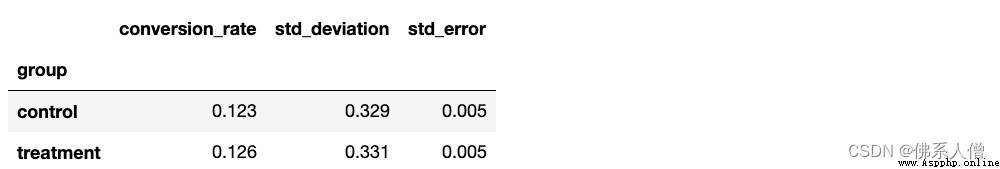
Start looking at our data :
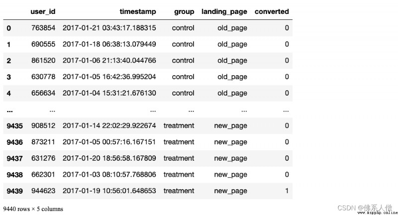
df = pd.read_csv('ab_data.csv')
df.head()
Output :
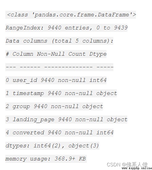
df.info()
Output :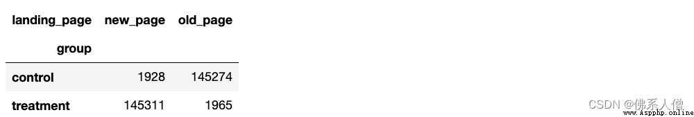
DataFrame There is 294478 That's ok , Each line represents a user session , as well as 5 Column :
user_id- Users per session ID
timestamp- Timestamp of the session
group- Which group of the session the user is assigned to { control Group , treatment Group }
landing_page- The design that each user sees in this session { old_page( Old page ), new_page}( New page )
converted- Whether the session is converted (0= Not converted ,1= conversion )
We actually only use group and converted Column for analysis .
Before we continue to sample the data to get our subset , Let's make sure that no user is sampled multiple times .
Yes 3894 Users appear more than once . Because the quantity is very small , We will continue to move them from DataFrame Delete in , To avoid sampling the same user twice .
sers_to_drop = session_counts[session_counts > 1].index
df = df[~df['user_id'].isin(users_to_drop)]
print(f' The updated dataset now has {
df.shape[0]} Entries ')
sampling
Now our DataFrame Clean and tidy , We can continue and n=4720 Sample entries for each group . We can use pandas Of DataFrame.sample() Method to do this , It will perform simple random sampling for us .
Be careful random_state=22: If you want to operate on your own laptop , I have set it to reproduce the results : just random_state=22 Use... In your function , You should get the same example as me .
control_sample = df[df['group'] == 'control'].sample(n=required_n, random_state=22)
treatment_sample = df[df['group'] == 'treatment'].sample(n=required_n, random_state=22)
ab_test = pd.concat([control_sample, treatment_sample], axis=0)
ab_test.reset_index(drop=True, inplace=True)
ab_test
ab_test.info()
Look at the segmentation of the experimental group and the control group
ab_test['group'].value_counts()
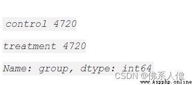
great !
3. Visualization results
conversion_rates = ab_test.groupby('group')['converted']
std_p = lambda x: np.std(x, ddof=0) # Std. Proportional deviation
se_p = lambda x: stats.sem(x, ddof=0) # Std. Proportional error (std / sqrt(n))
conversion_rates = conversion_rates.agg([np.mean, std_p, se_p])
conversion_rates.columns = ['conversion_rate', 'std_deviation', 'std_error']
conversion_rates.style.format ('{:.3f}')
From the above statistics , It seems that the performance of our two designs is very similar , Our new design performs a little better , about .12.3% Yes 12.6% Conversion rate of .
Visual code :
plt.figure(figsize=(8,6))
sns.barplot(x=ab_test['group'], y=ab_test['converted'], ci=False)
plt.ylim(0, 0.17)
plt.title( ' Conversion by group ', pad=20)
plt.xlabel('Group', labelpad=15)
plt.ylabel('Converted (proportion)', labelpad=15);
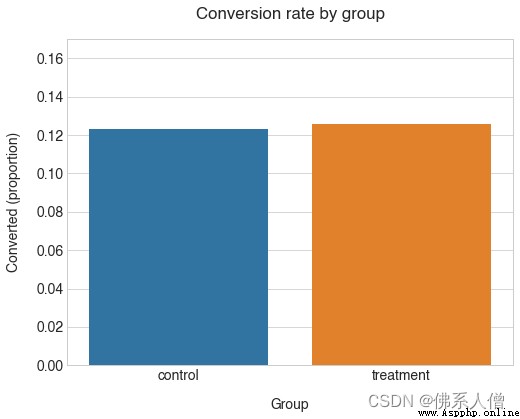
The conversion rate of our group is indeed very close . Attention, please. ,control Considering what we know about the average , The conversion rate of this group is lower than our expectation . Conversion rate (12.3% Yes 13%). This indicates that there are some differences in the results when sampling from the population .
therefore treatment The value of the group is higher . Is the difference statistically significant ?
4. Test the hypothesis
The final step in our analysis is to test our hypothesis . Because we have a very large sample , We can use the normal approximation to calculate our p value ( namely z test ).
Again ,Python Make all the calculations very easy . We can use the statsmodels.stats.proportion Module to get p Values and confidence intervals :
from statsmodels.stats.proportion import ratios_ztest, ratio_confint
control_results = ab_test[ab_test['group'] == 'control']['converted']
treatment_results = ab_test[ab_test['group'] == 'treatment']['converted']
n_con = control_results.count()
n_treat = treatment_results.count()
success = [control_results.sum(),treatment_results.sum()]
nobs = [n_con, n_treat]
z_stat, pval = ratios_ztest(successes, nobs=nobs)
(lower_con , lower_treat), (upper_con, upper_treat) = ratio_confint(successes, nobs=nobs, alpha=0.05)
print(f'z statistic: {
z_stat:.2f}')
print(f'p-value: {
pval:.3f }')
print(f'ci 95% for control group: [{
lower_con:.3f}, {
upper_con:.3f}]')
print(f'ci 95% for treatment group: [{
lower_treat:.3f}, {
upper_treat:.3f}]')
5. Come to the conclusion
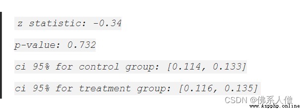
Because of our p -value=0.732 Much higher than ours α=0.05 threshold , We can't reject the null hypothesis Hₒ, This means that our new design is not significantly different from the old design ( Not to mention better )
Besides , If we look at this treatment Confidence interval of the group ([0.116, 0.135] or 11.6-13.5%), We will notice :
It includes us 13% Reference value of conversion rate
It does not include us 15% The target value ( Our goal is 2% The promotion of )
This means that the true conversion rate of the new design is more likely to be similar to our baseline , Not what we want 15% The goal of . This further proves that our new design is unlikely to be an improvement on the old design .