AdaBoost yes Boosting One of the algorithms , Well known , It can combine multiple weak classifiers into a strong classifier , Generally speaking, it means “ The Three Stooges , Zhuge Liang at the top ”. It requires weak classifiers to be good but different , The accuracy of each classifier should be within 50% above .
AdaBoos First initialize the sample weight distribution , A basic learning machine is trained from the initial training set , Then the weight distribution of the training samples is adjusted according to the classification results of the base learner , Regenerate into new base learners , Go ahead one by one , Until the requirements are met . The process is as follows :
(1) Initialize the sample weight distribution
(2) Generate basic classifiers G1
(3) Calculate classifier coefficients α \alpha α
(4) Update the weight distribution of training data
(5) Generate a new classifier G2
(6) loop (2-5)
(7) Add all classifiers linearly .
This process seems difficult to understand , There are too many formulas in the book , It's big , So let's take a simple example , This example is Li Hang 《 Statistical learning method 》 Inside . Suppose we have some data like this :
x x x Represents the sample value , y y y It is the label of these samples , What we have to do now is based on x Build a model to predict y Value . In essence, it is a binary classification problem , Build a classifier to classify these samples ,1 This is a positive example ,-1 Show counterexample . Before the official start , Let's assume the weights of these samples w w w It's all the same , All for 0.1( in total 10 Samples , The sum of the weights is 1), As shown in the following table :
The weight initialization code is as follows :
def func_w_1(x):
w_1=[]
for i in range(len(x)):
w_1.append(0.1)
return w_1
Suppose that our initial classifier can combine the previous n Samples are identified as positive examples , The remaining samples are counter examples , It can be expressed by the following formula : G i ( x ) = { 1 x<u − 1 x>u (1) Gi(x)= \begin{cases} 1& \text{x<u}\\ -1& \text{x>u} \end{cases}\tag{1} Gi(x)={ 1−1x<ux>u(1)
among u u u Threshold value , i i i It's a subscript ( Will not edit , crying ), For the convenience of discussion, we will u Is set to :
The code generated by the threshold is as follows :
def func_threshs(x):
threshs =[i-0.5 for i in x]
threshs.append(x[len(x)-1]+0.5)
return threshs
For each classifier G i ( x ) Gi(x) Gi(x), Its error rate e e e Use it to make an error ( namely G i ( x i ) ≠ y i Gi(xi)\neq yi Gi(xi)=yi) The weight sum of , For example, when the threshold is 2.5 when , The classifier is G i ( x ) = { 1 x<2.5 − 1 x>2.5 (2) Gi(x)= \begin{cases} 1& \text{x<2.5}\\ -1& \text{x>2.5} \end{cases}\tag{2} Gi(x)={ 1−1x<2.5x>2.5(2)
perhaps
G i ( x ) = { − 1 x<2.5 1 x>2.5 (3) Gi(x)= \begin{cases} -1& \text{x<2.5}\\ 1& \text{x>2.5} \end{cases}\tag{3} Gi(x)={ −11x<2.5x>2.5(3)
In this way, each threshold can be generated 2 A classifier , So there is 22 A classifier . For classifiers ( 2 ) (2) (2) A given input x x x, Its output G G G as follows
The code of classifier implementation is as follows :
def func_cut(threshs): y_pres_all={
}# Define a forward classifier , Shaped like a formula 2 y_last_all={
}# Define a forward classifier , Shaped like a formula 3
for thresh in threshs:
y_pres=[]
y_last=[]
for i in range(len(x)):
if x[i]<thresh:
y_pres.append(1)
y_last.append(-1)
else:
y_pres.append(-1)
y_last.append(1)
y_pres_all[thresh]=y_pres
y_last_all[thresh]=y_last
return y_pres_all,y_last_all
As can be seen from the table , sample 7、8、9 There's a mistake , Therefore, the error rate e=w7+w8+w9=0.3. We find this in the same way 22 Error rate of classifiers , Select the one with the lowest error rate as the base classifier . The code for calculating the error rate is as follows :
def sub_func_e(y,w_n,y_pres_all,thresh):
e=0
for i in range(len(y)):
if y_pres_all[thresh][i]!=y[i]:
e+=w_n[i];
return e
def sub_func_e_s(y,w_n,y_pres_all,threshs): e_s={
}
e_min=1
n=0
for thresh in threshs:
e=sub_func_e(y,w_n,y_pres_all,thresh)
e_s[thresh]=round(e,6)
if e<e_min:
e_min=round(e,6)
n=thresh
return e_s,e_min,n
def sub_func_e_all(y,w_n,y_pres_all,y_last_all,threshs):
e_s1,e_min1,n1=sub_func_e_s(y,w_n,y_pres_all,threshs)
e_s2,e_min2,n2=sub_func_e_s(y,w_n,y_last_all,threshs)
if e_min1<=e_min2:
return e_s1,e_min1,n1,y_pres_all
else:
return e_s2,e_min2,n2,y_last_all
In our case , By calculating all the error rates, the basic classifier is the formula 2 Shown . Let's start to calculate the coefficients of the classifier α \alpha α, Its calculation formula is as follows :
α = 1 2 l n 1 − e e (4) \alpha=\frac{1}{2}ln\frac{1-e}{e}\tag{4} α=21lne1−e(4) This shows the error rate e Not greater than 0.5, Otherwise, it will make α \alpha α<0. In this case α = 1 2 l n 1 − 0.3 0.3 = 0.4236 \alpha=\frac{1}{2}ln\frac{1-0.3}{0.3}=0.4236 α=21ln0.31−0.3=0.4236, The code for calculating the classifier coefficients is as follows :
def func_a_n(e_min):
a_n=round(0.5*math.log((1-e_min)/e_min),6)
return a_n
Finally, the weight distribution is updated according to the above calculation results w2, The updated formula is as follows :
w 2 i = w 1 ( i ) Z ∗ e − α i ∗ y i ∗ G 1 ( x i ) (5) w2i=\frac{w1(i)}{Z}*e^{-\alpha{i}*yi*G1(xi)}\tag{5} w2i=Zw1(i)∗e−αi∗yi∗G1(xi)(5) among Z = ∑ i = 1 m w 1 ( i ) ∗ e − α i ∗ y i ∗ G 1 ( x i ) (6) Z=\sum_{i=1}^m w1(i)*e^{-\alpha{i}*yi*G1(xi)}\tag{6} Z=i=1∑mw1(i)∗e−αi∗yi∗G1(xi)(6)
m It's the number of samples , It's not hard to see. Z Z Z The function of is to make the sum of the weights of the newly generated samples be 1, A new weight distribution can be obtained by this formula :
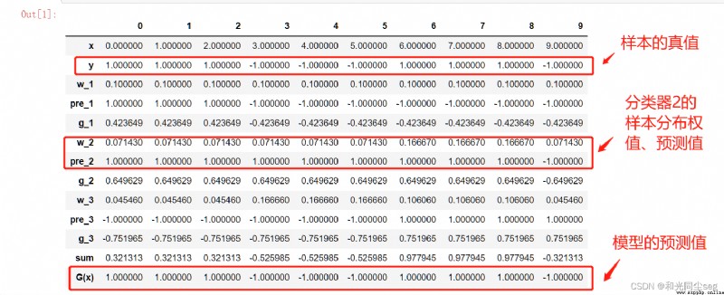
for instance , The weight of the first sample is updated to 0.07143, How did this come from , It's calculated like this : w 1 ( 1 ) Z ∗ e − α 1 ∗ y 1 ∗ G 1 ( x 1 ) = 0.1 5.50011 ∗ e − 0.4236 ∗ 1 ∗ 1 = 0.07143 , Its in Z = 0.07143 ∗ 7 + 0.16667 ∗ 3 = 5.50011 \frac{w1(1)}{Z}*e^{-\alpha{1}*y1*G1(x1)}=\frac{0.1}{5.50011}*e^{-0.4236*1*1}=0.07143, among Z=0.07143*7+0.16667*3=5.50011 Zw1(1)∗e−α1∗y1∗G1(x1)=5.500110.1∗e−0.4236∗1∗1=0.07143, Its in Z=0.07143∗7+0.16667∗3=5.50011, In fact, that is w2 And . It can be seen from the table that , The samples that were wrongly divided before 7,8,9 The weight of , The rest fell . The update code of sample distribution weight is as follows :
def func_w_n_tmp(x,pre_n,w_n,a_n):
w_n_tmp=[]
for i in range(len(x)):
w_new=round(w_n[i]*math.exp(-1*a_n*y[i]*pre_n[i]),6)
w_n_tmp.append(w_new)
return w_n_tmp
def func_z_n(w_n_tmp):
z_n=sum(w_n_tmp)
return z_n
def func_w_n(w_n_tmp,z_n):
w_n=[round(i/z_n,5) for i in w_n_tmp]
return w_n
We can use the same process to get multiple classifiers and the weight distribution of multiple classifiers , Together they form a new classifier , namely
G ( X ) = s i g n [ f ( x ) ] G(X)=sign[f(x)] G(X)=sign[f(x)] among
f ( x ) = α 1 ∗ G 1 ( x ) + α 2 ∗ G 2 ( x ) + ⋅ ⋅ ⋅ α n ∗ G n ( x ) f(x)=\alpha1*G1(x)+\alpha2*G2(x)+\cdot\cdot\cdot\alpha n*Gn(x) f(x)=α1∗G1(x)+α2∗G2(x)+⋅⋅⋅αn∗Gn(x)
s i g n [ f ( x ) ] sign[f(x)] sign[f(x)] Said when f ( x ) f(x) f(x) Greater than 0 You take 1, Less than 0 You take -1, Given in the book 3 Integration of classifiers , The result is f ( x ) = 0.4236 ∗ G 1 ( x ) + 0.6496 ∗ G 2 ( x ) + 0.7514 ∗ G 3 ( x ) f(x)=0.4236*G1(x)+0.6496*G2(x)+0.7514*G3(x) f(x)=0.4236∗G1(x)+0.6496∗G2(x)+0.7514∗G3(x), among : G 1 ( x ) = { 1 x<2.5 − 1 x>2.5 G1(x)= \begin{cases} 1& \text{x<2.5}\\ -1& \text{x>2.5} \end{cases} G1(x)={ 1−1x<2.5x>2.5 G 2 ( x ) = { 1 x<8.5 − 1 x>8.5 G2(x)= \begin{cases} 1& \text{x<8.5}\\ -1& \text{x>8.5} \end{cases} G2(x)={ 1−1x<8.5x>8.5 G 3 ( x ) = { − 1 x<5.5 1 x>5.5 G3(x)= \begin{cases} -1& \text{x<5.5}\\ 1& \text{x>5.5} \end{cases} G3(x)={ −11x<5.5x>5.5
be f ( x ) f(x) f(x) by f ( x ) = { 0.4236 + 0.6496 − 0.7514 = 0.3218 x<2.5 − 0.4236 + 0.6496 − 0.7514 = − 0.5254 2.5<x<5.5 − 0.4236 + 0.6496 + 0.7514 = 0.9774 5.5<x<8.5 − 0.4236 − 0.6496 + 0.7514 = − 0.3218 x>8.5 f(x)= \begin{cases} 0.4236+0.6496-0.7514=0.3218& \text{x<2.5}\\ -0.4236+0.6496-0.7514=-0.5254& \text{2.5<x<5.5}\\ -0.4236+0.6496+0.7514=0.9774& \text{5.5<x<8.5}\\ -0.4236-0.6496+0.7514=-0.3218& \text{x>8.5} \end{cases} f(x)=⎩⎪⎪⎪⎨⎪⎪⎪⎧0.4236+0.6496−0.7514=0.3218−0.4236+0.6496−0.7514=−0.5254−0.4236+0.6496+0.7514=0.9774−0.4236−0.6496+0.7514=−0.3218x<2.52.5<x<5.55.5<x<8.5x>8.5
The final classifier
G ( x ) = { 1 x<2.5 − 1 2.5<x<5.5 1 5.5<x<8.5 − 1 x>8.5 G(x)= \begin{cases} 1& \text{x<2.5}\\ -1& \text{2.5<x<5.5}\\ 1& \text{5.5<x<8.5}\\ -1& \text{x>8.5}\end{cases} G(x)=⎩⎪⎪⎪⎨⎪⎪⎪⎧1−11−1x<2.52.5<x<5.55.5<x<8.5x>8.5
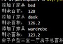
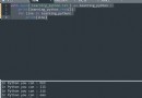
The output of the model is as follows :
The correct rate is 100%! Isn't that amazing ?
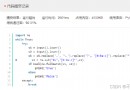
Finally we use python Achieve the results in the above example , We are like the book , Set up 3 A classifier , The specific implementation code is as follows :
# Import related libraries import math import pandas as pd import numpy as np # Input raw data x=[0,1,2,3,4,5,6,7,8,9] y=[1,1,1,-1,-1,-1,1,1,1,-1] T=3 # Set the number of classifiers # Initialize the sample weight distribution function def func_w_1(x): w_1=[] for i in range(len(x)): w_1.append(0.1) return w_1 # Generate threshold function def func_threshs(x): threshs =[i-0.5 for i in x] threshs.append(x[len(x)-1]+0.5) return threshs # Generate according to the threshold 22 The output of a classifier def func_cut(threshs): y_pres_all={
}
y_last_all={
}
for thresh in threshs:
y_pres=[]
y_last=[]
for i in range(len(x)):
if x[i]<thresh:
y_pres.append(1)
y_last.append(-1)
else:
y_pres.append(-1)
y_last.append(1)
y_pres_all[thresh]=y_pres # Forward classifier
y_last_all[thresh]=y_last # Backward classifier
return y_pres_all,y_last_all
# Find a classifier error rate e
def sub_func_e(y,w_n,y_pres_all,thresh):
e=0
for i in range(len(y)):
if y_pres_all[thresh][i]!=y[i]:
e+=w_n[i];
return e # Find the error rate of a class of classifiers def sub_func_e_s(y,w_n,y_pres_all,threshs): e_s={
}
e_min=1 n=0 for thresh in threshs: e=sub_func_e(y,w_n,y_pres_all,thresh) e_s[thresh]=round(e,6) if e<e_min: e_min=round(e,6) n=thresh return e_s,e_min,n # Find the error rate of two kinds of classifiers def sub_func_e_all(y,w_n,y_pres_all,y_last_all,threshs): e_s1,e_min1,n1=sub_func_e_s(y,w_n,y_pres_all,threshs) e_s2,e_min2,n2=sub_func_e_s(y,w_n,y_last_all,threshs) if e_min1<=e_min2: return e_s1,e_min1,n1,y_pres_all else: return e_s2,e_min2,n2,y_last_all # Output the best classifier def func_pre_n(y_all,n): pre_n=y_all[n] return pre_n # Find the error rate of the best classifier def func_a_n(e_min): a_n=round(0.5*math.log((1-e_min)/e_min),6) return a_n # Calculate the temporary distribution weight def func_w_n_tmp(x,pre_n,w_n,a_n): w_n_tmp=[] for i in range(len(x)): w_new=round(w_n[i]*math.exp(-1*a_n*y[i]*pre_n[i]),6) w_n_tmp.append(w_new) return w_n_tmp # seek Z def func_z_n(w_n_tmp): z_n=sum(w_n_tmp) return z_n # Calculate the weight of the updated sample distribution def func_w_n(w_n_tmp,z_n): w_n=[round(i/z_n,5) for i in w_n_tmp] return w_n # seek f(x) def func_g_n(x,pre_n,a_n): g_n=[] for i in range(len(x)): g_n_single=a_n*pre_n[i] g_n.append(g_n_single) return g_n # Each sub function is encapsulated def func_AdaBoost(x,y,T): a_n_s=[] # Save classifier coefficients w_n_s=[] # Save sample distribution weights pre_n_s=[] # Save the output of each base classifier e_n_s=[] # Save error rate g_n_s=[] # Save sub classifiers n_s=[] # Save threshold w_1=func_w_1(x) # Initialize the weight , All for 0.1 w_n_s.append(w_1) threshs=func_threshs(x) for i in range(T): w_n=w_n_s[i] y_pres_all,y_last_all=func_cut(threshs) e_s,e_min,n,y_all=sub_func_e_all(y,w_n,y_pres_all,y_last_all,threshs) pre_n=func_pre_n(y_all,n) a_n=func_a_n(e_min) w_n_tmp=func_w_n_tmp(x,pre_n,w_n,a_n) z_n=func_z_n(w_n_tmp) w_n=func_w_n(w_n_tmp,z_n) g_n=func_g_n(x,pre_n,a_n) a_n_s.append(a_n) w_n_s.append(w_n) pre_n_s.append(pre_n) g_n_s.append(g_n) n_s.append(n) e_n_s.append(e_min) return a_n_s,w_n_s,pre_n_s,g_n_s,n_s,e_n_s # The main program a_n_s,w_n_s,pre_n_s,g_n_s,n_s,e_n_s=func_AdaBoost(x,y,T) # list 、 Show results data={
'x':x,'y':y,'w_1':w_n_s[0],'pre_1':pre_n_s[0],'g_1':g_n_s[0],
'w_2':w_n_s[1],'pre_2':pre_n_s[1],'g_2':g_n_s[1],
'w_3':w_n_s[2],'pre_3':pre_n_s[2],'g_3':g_n_s[2]}
df=pd.DataFrame(data)
df['sum']=df['g_1']+df['g_2']+df['g_3']
# Output predicted value
df['G(x)']=np.sign(df['sum'])
df.T
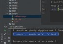
The output of the program is as follows :
remarks : The above code reference b standing up Lord “ Pay homage to the great God ”, Let's go and pay attention , Ha ha ha , It's gone. It's gone , Leave a message if you have any questions .