This article is based on the thesis published by my tutor and elder martial sister : Xue-Yang Min, Kun Qian, Ben-Wen Zhang, Guojie Song, and Fan Min, Multi-label active learning through serial-parallel neural networks, Knowledge-Based Systems (2022) Relevant papers can be viewed by yourself , This article is also mainly for the article algorithm learning and analysis , Finally, learn the code and self understanding
Catalog
Preface
1. Multi label concept preparation
1.1 What is multi label
1.2 Multi label model
1.3 Other contents of multiple labels
2.MASP Active learning in ( Learning scene )
2.1 Cold start
2.2 Active learning ( Additional queries )
2.3 Some query reasons in active learning
3.MASP The neural network in ( Learning models )
4. Multi label evaluation index
4.1 The bottleneck of traditional evaluation
4.2 Confuse matrix with parameter
4.3 Relevant evaluation schemes and curves
4.3.1 ROC Curve and AUC value
4.3.2 PR curve
4.3.3 F1 curve
5. The main framework of the program
5.1 The overview
5.2 test_active_learning function
5.3 Masp Constructors
5.4 MultiLabelData Constructors
5.5 MultiLabelAnn And ParallelAnn Constructors
6. List of representative functions
6.1 Learning on the Internet : one_round_train And bounded_train function
6.2 Cold start and active learning : two_stage_active_learn function
· About parameters
6.2.1 Cold start batch and active learning batch calculation
6.2.3 Cold start
6.2.4 Active learning
6.3 F1 The calculation of my_test And compute_f1
Epilogue
MASP The full name is Multi-label active learning through serial-parallel neural networks, It is a learning model and algorithm of neural network constructed by serial and parallel , And take active learning as a learning scenario to build an efficient algorithm for solving multi label learning problems
Most of the machine learning algorithms in my previous articles have focused on iris This dataset , as everyone knows , This data set has three labels
@RELATION iris
@ATTRIBUTE sepallength REAL
@ATTRIBUTE sepalwidth REAL
@ATTRIBUTE petallength REAL
@ATTRIBUTE petalwidth REAL
@ATTRIBUTE class {Iris-setosa,Iris-versicolor,Iris-virginica}
In the learning process, it is necessary to predict the unique label of a certain data row , This should be a multi classification problem , For example, the following iris Three data rows of , Their correct label is "Iris-setosa" This inference
4.3,3.0,1.1,0.1,Iris-setosa
5.8,4.0,1.2,0.2,Iris-setosa
5.7,4.4,1.5,0.4,Iris-setosa
However, in the field of machine learning, there is a multi label situation in label prediction , In the multi label problem , The label of a data row is not so single , It may be the following . Each attribute column can have multiple cases , This is a case of multi label . therefore , Assume that the total number of tags is \(L\), It is not difficult to find that the tag possibility of an attribute line is \(2^L\).
4.3,3.0,1.1,0.1,Iris-setosa,Iris-versicolor
5.8,4.0,1.2,0.2,Iris-virginica
5.7,4.4,1.5,0.4,Iris-versicolor,Iris-virginica
6.4,3.1,5.5,1.8,None
6.0,3.0,4.8,1.8,Iris-setosa,Iris-virginica
therefore , Assume that the total number of tags is \(L = 1\), So usually when \(L=1\), Yes \(2^1\), It is a binary classification problem , That is to say, the data row is non 1 namely 0 Binary assertion of , AdaBoost The single classifier in is to achieve this operation , It is also the simplest classifier .
When \(L > 1\) Is a common multi label problem , At this point, if the restricted label selection is mutually exclusive , Then we return to the common multi classification problem .
When we talked about multi classification problems, we had a fixed \(N \times 1\) Label column , The range of stored values is 0~\(L-1\) , Used to indicate a certain label . If you enter the multi label field , This stored value " Column " It should be expanded into a " matrix ", Which is a \(N \times L\) Label matrix to store . This is related to the size of the part in the dataset where instances are stored \(N \times M\) The matrix of forms a two tuple :\[S=(\mathbf{X}, \mathbf{Y}) \tag{1}\]
among :
Here, each tag value is not as much as it can be taken in the multi classification problem , Basically, Boolean means more , A common dataset defines \(y_{ij}=1\) Express , \(y_{ij}=-1\) It means nothing . Of course, in some other cases \(y_{ij}=0\) To represent the absence . It's understandable , After all, in real life, there are more uncertain data than certain data , Easy access to data , But be clear about what it means , Or take the time to define what it means , In fact, it's a complicated thing . This is also the active learning later (Active Learning) One of the reasons why it started .
Multiple tags have some related features , For example, the problem of label relevance , This is a part that many multi label algorithms need to consider , Many common algorithms will cut in from different angles , For example, there are : Regardless of relevance 、 Consider pairwise correlations 、 Consider more than two tag dependencies . for example BP-MLL What we are thinking about is twoness , and LIFT The algorithm discards the correlation .
BP-MLL original text : Zhang, M.-L., & Zhou, Z.-H. (2006). Multi-label neural networks with applications to functional genomics and text categorization. IEEE transactions on Knowledge and Data Engineering, 18, 1338–1351.
There is a blog about my teacher : BP-MLL
LIFT original text : Zhang, M.-L., & Wu, L. (2014). LIFT: Multi-label learning with label-specific features. IEEE Transactions on Pattern Analysis and Machine Intelligence, 37, 107–120.
There is a blog about my teacher : LIFT
In addition, the tag value can also be [0,1] The probability value of the multi label study , Not Boolean , This is it. Label distribution learning problem
For more information on this part, see Lecture version of multi label learning ( Internal discussion , To be continued )_ Min fan's blog -CSDN Blog
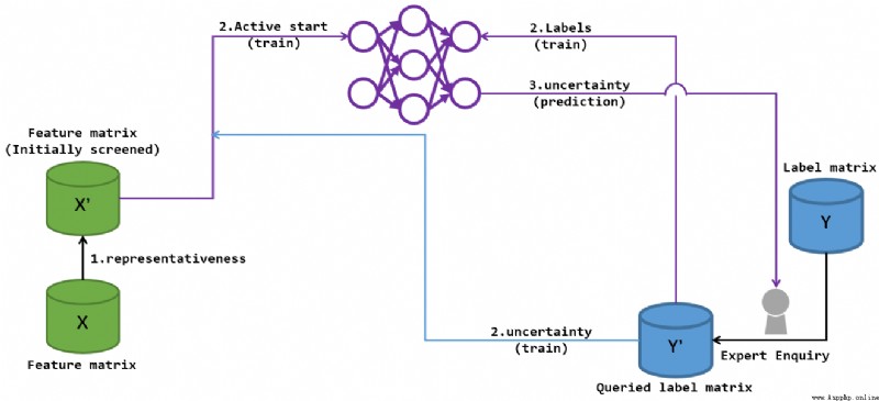
Through the above multi label missing phenomenon and the coincidence of active learning motivation , It can be found that active learning with multiple tags should be possible . MASP The following model is proposed in : Limited budget cold start multi label learning
In general, such a process , All the parts that need the assistance of the target label matrix are completed by the expert query , This is the core of active learning ( The code is reflected in the query of the target matrix ) The most special thing in this process is the intervention of cold start , Cold start ensures the formation of the basic neural network , It is convenient for us to extract some untrained tag information later , So as to further deepen the characteristics of the back feeding network . I try to use two pictures to describe this process .
This picture illustrates 2,3 Cold start phase of step , In the picture \(Y^{\prime}\) It is based on... With the participation of experts \(X\) Marked label matrix , The number of rows of this matrix is smaller than that of all label matrices \(Y\) Of , but \(Y\) Is the unknowable part , Therefore, it is known that \(Y^{\prime}\) It will provide guidance for the next study . In the picture \(X^{\prime}\) For the characteristic matrix \(X\) From pretreatment .
This preprocessing results in the training data row set \(U\), And through the data marked by professionals sparsity( sparse ) The high value label determines the data column \(V\), Finally, the cold start query tag point set \(\{(i,j)|i \in U, j \in V\}\). Then when training the network , \(Y^{\prime}\) The tag provided will be learned as the goal of network loss function fitting . Finally, it passes a finite number of times batch Training , Get an evaluation parameter : uncertainty (uncertainty). This parameter can once again guide experts to mark more key tags , So as to further promote \(Y\) To \(Y^{\prime}\) The transformation of , perfect \(Y^{\prime}\).
Cold start phase sparsity There is a certain meaning of active learning in the introduction of , But then uncertainty The characteristics of active learning are more obvious in the process of repeated refreshing :
Provided after the cold start of the last round "uncertainty" The information has pushed the experts to further improve \(Y^{\prime}\), Nature has also expanded \(X^{\prime}\) The queryable set of , So according to the new \(S^{\prime} = \mathbf{X^{\prime}}, \mathbf{Y^{\prime}}\) Further training network . After training, we get new uncertainty Further guide experts to label , To update \(Y^{\prime}\), So as to form a training -> Get new uncertainty-> Training ... The cycle of . Until the expert query reaches the upper limit , Output final forecast .
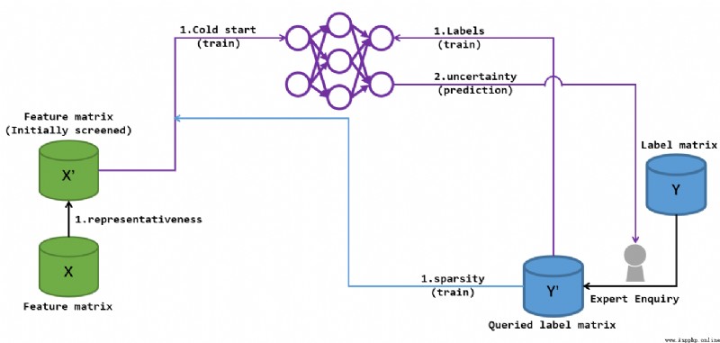
MASP Medium SP Describes the network it uses ——serial-parallel neural networks. Here I use the original picture in the paper to describe :
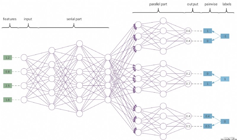
So called serial (serial) The Internet Is the leading in the figure serial part, This part of the network plays the role of feature extraction , All the features between tags are analyzed in series here , At the same time, it also realizes the processing of label correlation . therefore MASP The tag correlation is considered in , However, the feature of this paper is that the consideration of label relevance is completed in the pilot learning , Instead of analyzing the predicted results , It is different from the common tag correlation processing methods .
parallel (parallel) The network is the part of the network before parallel output in the figure , The number of this part of the network is equal to \(L\), The implication , Each parallel network implements a separate binary prediction for a tag . MASP The output of the parallel network used in is a dual port output , The output values range from [0,1], When the network makes predictions , As a positive output structure , We define that most of the dual ports are evaluated as 1, The smaller part is evaluated as 0. Final pairwise = <1, 0> Is predicted to be a negative label (-1), That is, the label does not exist ; Final pairwise = <0, 1> When predicted as a positive label (1). Another available solution is to use softmax Calculate the dual port as a certain probability value , The probability of being a positive label , Finally, some thresholds are determined to determine the positive and negative of the current tag .
When training on the Internet , As a negative backPropagation Structure of , If the target tag is a negative tag (-1), Then create a pairwise = <1, 0>, During training forward The loss function is then calculated for this pairwise To fit the dual port ; If the target label is a positive label (1), Then create a pairwise = <0, 1>, Fitting is the same . Additional emphasis , When the target tag is missing (0), The algorithm will generate pairwise = <\(\hat{y}_{0}\), \(\hat{y}_{1}\)>, Thus, there is no penalty in calculating the loss function . This is it. MASP There is no penalty for missing tags in Characteristics of .
say concretely , Code emulation MASP when , The missing tag does not mean that the tag is in the dataset \(Y\) Is missing , But this label is not marked by experts , That is to say \(Y^{\prime}\) Could not find this tag in . Of course , Although it is missing , But it can still be predicted by mature networks , Or it will be selected as uncertainty The label is thus marked by experts ( The representation in the code is queried ) Thus becoming a non missing tag .
In addition, I get some network information by reading the source code , MASP In the backPropagation The gradient descent scheme for the loss function is Adaptive moment estimation (Adam: Adaptive Moment Estimation), The activation functions of most layers use Sigmoid, But between the serial and parallel networks ReLU, The ultimate loss function is MSE Mean square error .
MASP Adopted F1 The evaluation index , about F1, AUC Readers who know about it can read it directly 4.3.3
There is only one label column in the multi classification problem , Whether the prediction is correct can be used 1/0 Express , After extending to multiple data rows, you can judge 1 The proportion of is recognized , This is it. accuracy.
But in the multi label problem, a data row has multiple label columns , If 1/0 If the prediction is correct, there will be some unreasonable things : Firstly, the label correctness of multi label problem is Boolean , A tag predicts " non-existent / There is " It may all be reasonable , For example, for a \(L=4\) The data line , If the truth is {+1, -1, -1, -1}, I can never say that the prediction is { +1, -1, +1, -1} Absolutely wrong , Because after all, I predicted three ! Well, in proportion , For example, this data line predicts accuracy by 75%. But it doesn't make sense , Because the multi label matrix in the multi label data in reality has serious Label sparsity , Simply put, the number of negative labels in a data row may account for more than 90% of all labels ! In this way, it seems that if I predict all the labels of a data row as negative labels 99% The accuracy of , however , Is that reasonable? ? No matter what picture I give you , Let you predict what animals , You all predict " There are no animals ".
Therefore, we need to put forward some new evaluation indicators .
Confusion matrix is a very key thing to evaluate the overall accuracy , It is also the basis of various evaluation indicators :
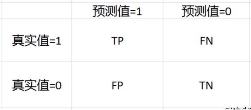
The overlapping parts in the table give rise to four overlapping situations between the forecast and the actual :
Through these four information, several corresponding indicators have been born :
Many evaluation indicators have been derived from the above three indicators , Here are a few .
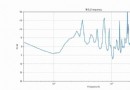
First of all ROC curve , Full name “ Subject curve ”, Simply speaking , He will continue to increase with the deepening of the survey sample TPR and FPR As ordinate and abscissa respectively . When actually looking at this image, please do not understand it as a function image , Look at it as a map , and (0,0) There is a traveler , He can only go north or East in each round , But no matter how he goes, he will eventually come to (1,1) spot . This understanding can perfectly interpret the connotation of the above purple characters .

so ROC A curve is a gradient line , But with the increase of samples , Our curves will also become smoother . meanwhile , When this curve " The more convex " when , It proves that TPR The increase of is very fast , In other words, the traveler went north as much as possible at the beginning , Finally, there is no alternative but to arrive (1,1) So I went east . We are hoping for such a result , Just put TPR From the example of catching criminals , If the robbers can be caught in the first few trials , It seems that we can end the arrest ahead of time and avoid the remaining unjust, false and wrong cases . So in order to measure " Convex " The degree of , We define this curve at [0,1] Definite integral value on ( area ) by AUC value , As an index to judge whether the sample distribution is good or bad .
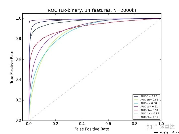
If the first extraction \(x\) Samples are predicted to be positive, and all predictions are correct , And just put all \(x\) All the real positive samples have been predicted , that TPR before \(x\) The score will change from \(\frac{0}{x}\) Become directly \(\frac{x}{x}\), This is it. best Of ROC curve , His AUC The value is 1.
Learn by introduction , Precision The initial value of is from 1 Start (Precision The value starts with \(\frac{0}{1}\)) The possibility is relatively small , Because we often rank the probability of positive samples when we actually make predictions , Often the probability that the prediction of the first sample is positive is close to 100%), Then, with the occurrence of errors in the prediction process, it leads to gradual deviation 1, But because molecules have accumulated amounts , So it won't come to 0. and Recall The value will change from 0 To approach gradually 1, When the sample distribution is orderly , This approach will reach... Earlier . Final , With Recall Abscissa , Precision Vertical coordinates , To get PR curve .
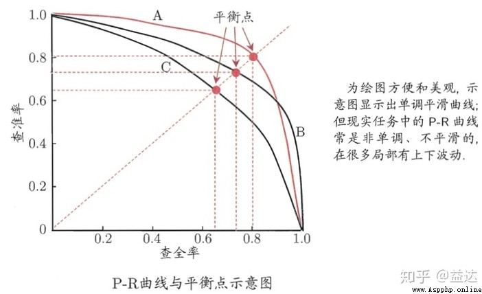
For different models, the prediction effect on the same data set is better , We can draw a series of PR curve , In general, if a curve is completely “ Surround ” Another curve , We can think that the classification effect of this model is better than that of the contrast model . however PR The description of the curve is rough after all , Actually about Precision And Recall We use more F1, This is also MASP One of the measurement schemes selected in .
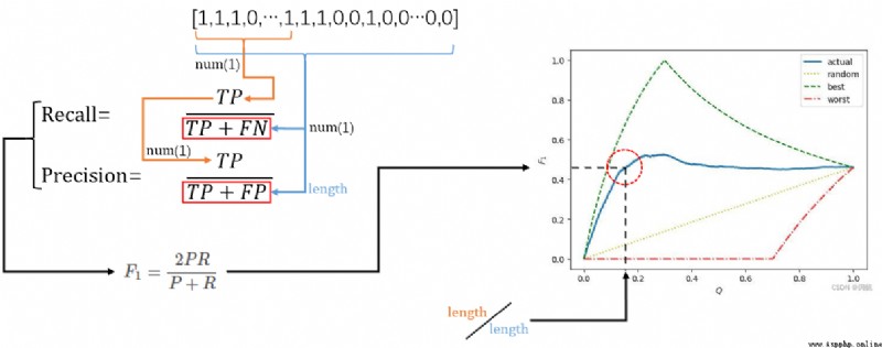
F1 The value is P and R Of the harmonic mean of 2 times :\[F_{1} = \frac{2PR}{P+R} \tag{4}\] here P representative Precision, R representative Recall.
In fact, we get the final predicted tag value through network learning or other means , In the beginning, these tag values have not been converted to certain 1/-1 When they are both a dual port value <\(\hat{y}_{0}\), \(\hat{y}_{1}\)> (\(\hat{y}_{p} \in [0,1]\)), And uniquely correspond to its real tag value in logic . Logically, these Separate dual port binary And Its true tag value But they are all coordinates in the label matrix \(\{(i,j)| 0 \leq i < N , 0 \leq j < L\}\) Of mapping and Value . Now I reduce them all to one-dimensional arrays , This correspondence remains unchanged , Then I will Real tag value The basis for carrying out Dual port binary softmax Probability value Sort , That is, according to the probability that the labels trained by the network may be positive Real label Rearrange , Get one Real label Rearranging arrays sortedArray( Array length is N*L, It's about [1,1,1,...,1,1, -1,-1,-1,...,-1,-1], But because the predictions are flawed , There may be continuous 1 Mixed with -1, continuity -1 Mixed with 1). Then keep taking it out sortedArray Before \(Q\%\) data , And they all predict that the data in this data is a positive label , And then according to the formula 4 To calculate F1.
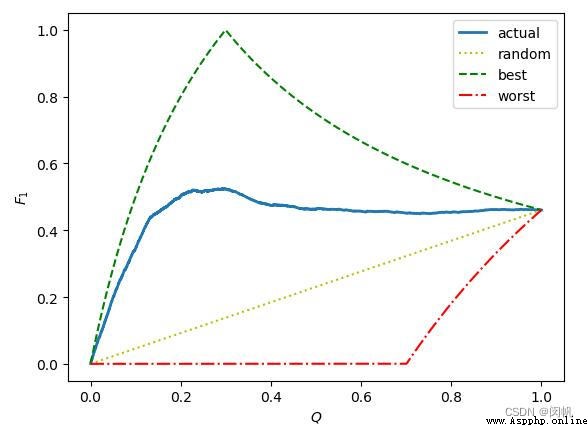
best The curve of represents the best F1 curve , If the current total amount of data is \(x+y\), among \(x\) One is a real positive sample , \(y\) One is a real negative sample . We can judge by the formula , In the best case before \(x\) The sample is indeed a positive sample , So before \(x\) In secondary sampling Precision Will always be 1( Take a forecast as a positive prediction pair ), And when the forecast goes into the \(x+1\) When a data Precision Will be taken from 1 falling ( There are no positive samples , Another positive prediction will lead to wrong prediction ), Until it finally drops to \(\frac{x}{x+y}\). and Recall At the beginning \(\frac{0}{x}\), As sampling continues \(\frac{1}{x}\),\(\frac{2}{x}\)... increase . And then after checking the \(x\) Data changes to \(\frac{x}{x} = 1\), It will not change in the future . So when checking to the \(x\) When a data , Precision Is the last time for 1, and Recall For the first time 1, So you get best Above picture best The highest value of the curve :\(F_{1} = \frac{2 \times 1 \times 1}{1+1} = 1\). Before [0~\(x\)] Within the interval Precision keep 1 unchanged , and Recall It is another step from 0->1 The increasing process of , Therefore, the curve in the figure is increasing .
The actual data will be blue actual curve , although [0~\(x\)] The interval will be incremented by a part , however Precision It is possible that some wrong predictions may lead to early departure from 1 Start to fall , and Recall It will also slow down due to the increase of wrong predictions . So the blue line will deviate in advance best curve , Reach ahead of time Peak And fall , Finally, at the end, a small number of successful predictions lead to Recall Rise to slightly raise F1. Last on worst And random Curve readers can make a similar analysis , in short worst In fact, it is the result of sorting negative labels first and then positive labels .
In the end, no matter how much trouble , Finally, after the global data test Recall It must be 1, Precision It must be \(\frac{x}{x+y}\). So the final curve finally converges on \((1.0,\frac{2x}{2x+y})\)( Junior high school mathematics calculation )
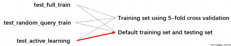
The volume of source code is relatively large , Several rounds of tests were conducted , The scene is divided into supervised learning , Semi supervised learning and active learning of random query . In terms of training data , There are by 5 Fold cross validation to use only one training set to complete training and testing , There is also training given using the default raw data set / Test documents to guide the test and training respectively . Here, for the sake of simplicity, we mainly show a branch :
In the specific description, I will omit some code for reading and writing files , The functions of some variables will be introduced in the description , At the end of the paper, some common variables are explained . This time it's not my normal article , I will The top-down Introduce this code , First put the main body , When it comes to a certain function, I am simply explaining . Please check the source code if you are interested .
The data used in this article to describe the test is Birds Data sets :
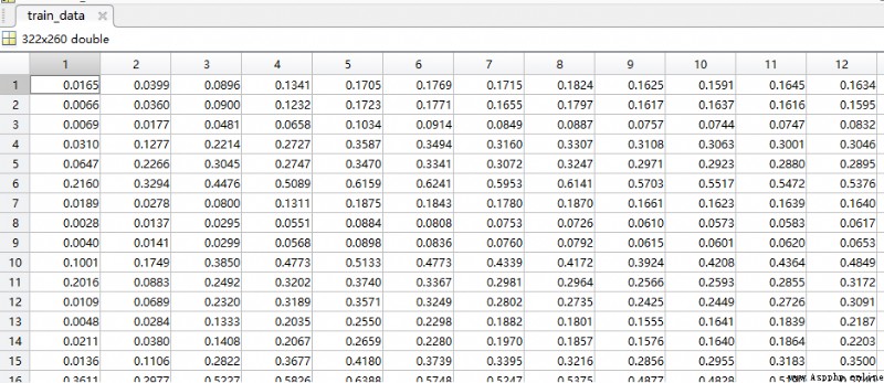
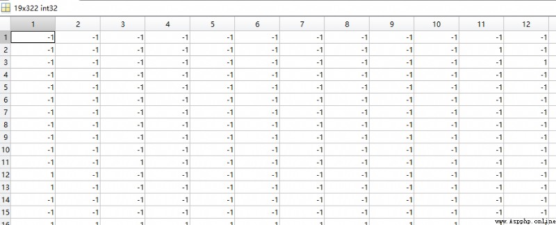
( The test matrix is not shown , Yes 323 Test data , The number of test and training data sets is almost the same )
I use a diagram to describe the specific process
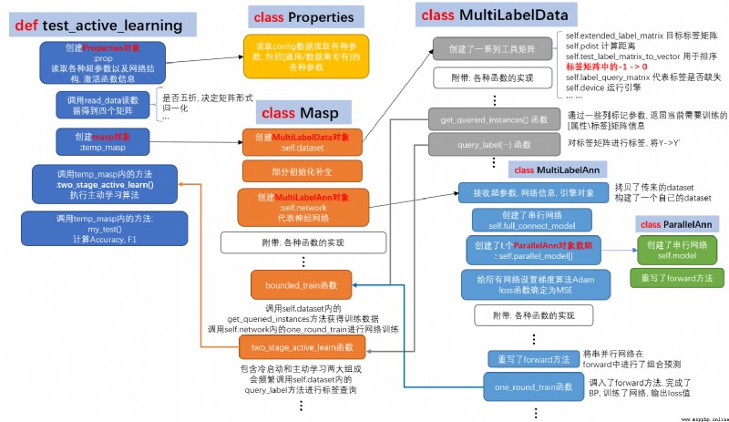
Each color in this diagram represents a class , Except for the leftmost function , You can take test_active_learning As part of this process main Function to understand . The vertical same color flow box of all classes represents the process of task completion in this class constructor , And in the " Incidental : Various Implementation of function " Below the white box are some key function members of this class , Without this white box, all the methods owned by the current class have been displayed . obviously , Only ParallelAnn and Properties Class coincidence , Because their volume is the smallest . The other three classes are relatively large , There are many incidental methods , It is impossible and unnecessary for this article to introduce , I will only make a basic exposition of some key points . If you are interested, please check the source code .
def test_active_learning(para_dataset_name: str = 'Emotion'):
"""
Used to fill in the third set of experimental data , Compared with the general multi label learning active algorithm .
:param para_dataset_name: Dataset name .
"""
print(para_dataset_name)
temp_start_time = time.time()
prop = Properties(para_dataset_name)
temp_train_data, temp_train_labels, temp_test_data, temp_test_labels = read_data(para_train_filename=prop.filename, param_cross_flag=False)
prop.train_data_matrix = temp_train_data
prop.test_data_matrix = temp_test_data
prop.train_label_matrix = temp_train_labels
prop.test_label_matrix = temp_test_labels
prop.num_instances = prop.train_data_matrix.shape[0]
prop.num_conditions = prop.train_data_matrix.shape[1]
prop.num_labels = prop.train_label_matrix.shape[1]
prop.full_connect_layer_num_nodes[0] = prop.num_conditions
temp_masp = Masp(para_train_data_matrix=prop.train_data_matrix,
para_test_data_matrix=prop.test_data_matrix,
para_train_label_matrix=prop.train_label_matrix,
para_test_label_matrix=prop.test_label_matrix,
para_num_instances=prop.num_instances,
para_num_conditions=prop.num_conditions,
para_num_labels=prop.num_labels,
para_full_connect_layer_num_nodes=prop.full_connect_layer_num_nodes,
para_parallel_layer_num_nodes=prop.parallel_layer_num_nodes,
para_learning_rate=prop.learning_rate,
para_mobp=prop.mobp, para_activators=prop.activators)
temp_init_end_time = time.time()
temp_masp.two_stage_active_learn(para_instance_selection_proportion=prop.instance_selection_proportion,
para_budget=prop.budget,
para_cold_start_labels_proportion=prop.cold_start_labels_proportion,
para_label_batch=prop.label_batch,
para_instance_batch=prop.instance_batch,
para_dc=prop.dc, para_pretrain_rounds=prop.pretrain_rounds,
para_increment_rounds=prop.increment_rounds,
para_enhancement_threshold=prop.enhancement_threshold)
temp_acc, temp_f1 = temp_masp.my_test()
temp_test_end_time = time.time()
print('Init time: ', temp_init_end_time - temp_start_time)
print('Cold start time: ', temp_masp.cold_start_end_time - temp_init_end_time)
print('One round time: ', (temp_masp.multi_round_end_time - temp_masp.cold_start_end_time)/temp_masp.num_additional_queries)
print('Bounded time: ', temp_masp.final_update_end_time - temp_masp.multi_round_end_time)
print('Test time: ', temp_test_end_time - temp_masp.final_update_end_time)class Masp:
"""
Multi-label active learning through serial-parallel networks.
The main algorithm.
"""
def __init__(self, para_train_data_matrix, para_test_data_matrix, para_train_label_matrix, para_test_label_matrix, # Four matrices
para_num_instances: int = 0, para_num_conditions: int = 0, para_num_labels: int = 0, # The three parameters of the matrix
para_full_connect_layer_num_nodes: list = None, para_parallel_layer_num_nodes: list = None,
para_learning_rate: float = 0.01, para_mobp: float = 0.6, para_activators: str = "s" * 100):
# Step 1. Accept parameters.
self.dataset = MultiLabelData(para_train_data_matrix=para_train_data_matrix,
para_test_data_matrix=para_test_data_matrix,
para_train_label_matrix=para_train_label_matrix,
para_test_label_matrix=para_test_label_matrix,
para_num_instances=para_num_instances, para_num_conditions=para_num_conditions,
para_num_labels=para_num_labels)
self.representativeness_array = np.zeros(self.dataset.num_instances)
self.representativeness_rank_array = np.zeros(self.dataset.num_instances)
self.output_file = None
self.device = torch.device('cuda')
self.network = MultiLabelAnn(self.dataset, para_full_connect_layer_num_nodes, para_parallel_layer_num_nodes,
para_learning_rate, para_mobp, para_activators, self.device).to(self.device)
self.cold_start_end_time = 0
self.multi_round_end_time = 0
self.final_update_end_time = 0
self.num_additional_queries = 0stay test_active_learning A... Is declared in the function Masp object , This class describes the main process of the algorithm
class MultiLabelData:
"""
Multi-label data.
This class handles the whole data.
"""
def __init__(self, para_train_data_matrix, para_test_data_matrix, para_train_label_matrix, para_test_label_matrix,
para_num_instances: int = 0, para_num_conditions: int = 0, para_num_labels: int = 0):
"""
Construct the dataset.
:param para_train_filename: The training filename.
:param para_test_filename: The testing filename. The testing data are not employed for testing.
They are stacked to the training data to form the whole data.
:param para_num_instances:
:param para_num_conditions:
:param para_num_labels:
"""
# Step 1. Accept parameters.
self.num_instances = para_num_instances
self.num_conditions = para_num_conditions
self.num_labels = para_num_labels
self.data_matrix = para_train_data_matrix
self.label_matrix = para_train_label_matrix
self.test_data_matrix = para_test_data_matrix
self.test_label_matrix = para_test_label_matrix
# -1 to 0
self.test_label_matrix[self.test_label_matrix == -1] = 0
self.label_matrix[self.label_matrix == -1] = 0
self.test_label_matrix_to_vector = self.test_label_matrix.reshape(-1) # test label matrix n*l to vector
self.extended_label_matrix = np.zeros((self.num_instances, self.num_labels * 2))
for i in range(self.num_instances):
for j in range(self.num_labels):
# Copy label matrix.
if self.label_matrix[i][j] == 0:
self.extended_label_matrix[i][j * 2] = 1
self.extended_label_matrix[i][j * 2 + 1] = 0
else:
self.extended_label_matrix[i][j * 2] = 0
self.extended_label_matrix[i][j * 2 + 1] = 1
# Step 2. Space allocation for other member variables.
self.test_predicted_proba_label_matrix = np.zeros((self.num_instances, self.num_labels))
self.predicted_label_matrix = np.zeros((self.num_instances, self.num_labels))
self.test_predicted_label_matrix = np.zeros(self.test_label_matrix.size)
self.label_query_matrix = np.zeros((self.num_instances, self.num_labels))
self.has_label_queried_array = np.zeros(self.num_instances)
self.label_query_count_array = np.zeros(self.num_labels)
self.distance_measure = MyEnum.EUCLIDEAN
self.device = torch.device('cuda')
self.pdist = torch.nn.PairwiseDistance(p=2, eps=0, keepdim=True).to(self.device)
Just mentioned , MultiLabelData The member variables declared in the class are various tags that may be used in various stages of the algorithm [ Array / matrix ], Bucket array , The staging [ Array / matrix ] And various operations acting on these structures . Is different from Properties Class , Established , Super parameters for regulation .

class MultiLabelAnn(nn.Module):
"""
Multi-label ANN.
This class handles the whole network.
"""
def __init__(self, para_dataset: MultiLabelData = None, para_full_connect_layer_num_nodes: list = None,
para_parallel_layer_num_nodes: list = None, para_learning_rate: float = 0.01,
para_mobp: float = 0.6, para_activators: str = "s" * 100, para_device=None):
"""
:param para_dataset:
:param para_full_connect_layer_num_nodes:
:param para_parallel_layer_num_nodes:
:param para_learning_rate:
:param para_mobp:
:param para_activators:
:param para_device:
"""
super().__init__()
self.dataset = para_dataset
self.num_parts = self.dataset.num_labels
self.num_layers = len(para_full_connect_layer_num_nodes) + len(para_parallel_layer_num_nodes)
self.learning_rate = para_learning_rate
self.mobp = para_mobp
self.device = para_device
temp_model = []
for i in range(len(para_full_connect_layer_num_nodes) - 1):
temp_input = para_full_connect_layer_num_nodes[i]
temp_output = para_full_connect_layer_num_nodes[i + 1]
temp_linear = nn.Linear(temp_input, temp_output)
temp_model.append(temp_linear)
temp_model.append(get_activator(para_activators[i]))
self.full_connect_model = nn.Sequential(*temp_model)
temp_parallel_activators = para_activators[len(para_full_connect_layer_num_nodes) - 1:]
self.parallel_model = [ParallelAnn(para_parallel_layer_num_nodes, temp_parallel_activators).to(self.device)
for _ in range(self.dataset.num_labels)]
self.my_optimizer = torch.optim.Adam(itertools.chain(self.full_connect_model.parameters(),
*[model.parameters() for model in self.parallel_model]),
lr=para_learning_rate)
self.my_loss_function = nn.MSELoss().to(para_device)
class ParallelAnn(nn.Module):
"""
Parallel ANN.
This class handles the parallel part.
"""
def __init__(self, para_parallel_layer_num_nodes: list = None, para_activators: str = "s" * 100):
super().__init__()
temp_model = []
for i in range(len(para_parallel_layer_num_nodes) - 1):
temp_input = para_parallel_layer_num_nodes[i]
temp_output = para_parallel_layer_num_nodes[i + 1]
temp_linear = nn.Linear(temp_input, temp_output)
temp_model.append(temp_linear)
temp_model.append(get_activator(para_activators[i]))
self.model = nn.Sequential(*temp_model)
MultiLabelData Class is in charge of a series of operations such as network construction and operation . Most of the content uses torch Programming content .
one_round_train The function is located at MultiLabelAnn class , It is used to realize once forward+backPropagation The process of , Because it's used here torch Programming , So it's very concise ( The wheels are so fragrant !). What is the kernel of the wheel? Welcome to my blog : be based on Java Self study notes of machine learning ( The first 71-73 God :BP neural network )_LTA_ALBlack The blog of -CSDN Blog
 def one_round_train(self, para_input: np.ndarray = None, para_extended_label_matrix: np.ndarray = None, para_label_query_matrix: np.ndarray = None) -> object:
"""
One round train. Use instances with labels.
:return:
"""
temp_outputs = self(para_input)
temp_memory_outputs = temp_outputs.cpu().data
para_extended_label_matrix = torch.tensor(para_extended_label_matrix, dtype=torch.float)
i_index, j_index = np.where(para_label_query_matrix == 0)
para_extended_label_matrix[i_index, j_index * 2] = temp_memory_outputs[i_index, j_index * 2]
para_extended_label_matrix[i_index, j_index * 2 + 1] = temp_memory_outputs[i_index, j_index * 2 + 1]
temp_loss = self.my_loss_function(temp_outputs, para_extended_label_matrix.to(self.device))
self.my_optimizer.zero_grad()
temp_loss.backward()
self.my_optimizer.step()
return temp_loss.item()
def forward(self, para_input: np.ndarray = None):
temp_input = torch.as_tensor(para_input, dtype=torch.float).to(self.device)
temp_inner_output = self.full_connect_model(temp_input)
temp_inner_output = [model(temp_inner_output) for model in self.parallel_model]
temp_output = temp_inner_output[0]
for i in range(len(temp_inner_output) - 1):
temp_output = torch.cat((temp_output, temp_inner_output[i + 1]), -1)
return temp_output
This function needs to pass three parameters , One is Attribute matrix to be trained , be used for forward Provides input neurons ; The other is Extended target label matrix , be used for BackPropagation Calculate the loss function and prepare for quantifying the penalty information to update the network edge weight ; And finally Whether the tag matrix is missing the tag matrix , It is specially introduced in training to take out the missing labels when calculating the loss function " Take care of alone ", The loss is guaranteed to be 0, No punishment
 def bounded_train(self, para_lower_rounds: int = 200, para_checking_rounds: int = 200,
para_enhancement_threshold: float = 0.001):
temp_input, temp_extended_label_matrix, temp_label_query_matrix = self.dataset.get_queried_instances()
print("bounded_train")
# Step 2. Train a number of rounds.
for i in range(para_lower_rounds):
if i % 100 == 0:
print("round: ", i)
self.network.one_round_train(temp_input, temp_extended_label_matrix, temp_label_query_matrix)
# Step 3. Train more rounds.
i = para_lower_rounds
temp_last_training_accuracy = 0
while True:
temp_loss = self.network.one_round_train(temp_input, temp_extended_label_matrix, temp_label_query_matrix)
if i % para_checking_rounds == para_checking_rounds - 1:
temp_training_accuracy, temp_testing_accuracy, temp_overall_accuracy = self.network.test()
print("Regular round: ", (i + 1), ", training accuracy = ", temp_training_accuracy)
if temp_last_training_accuracy > temp_training_accuracy - para_enhancement_threshold:
break # No more enhancement.
else:
temp_last_training_accuracy = temp_training_accuracy
print("The loss is: ", temp_loss)
i += 1
temp_training_accuracy, temp_testing_accuracy, temp_overall_accuracy = self.network.test()
print("Training accuracy (learner knows it) = ", temp_training_accuracy,
", testing accuracy (learner does not know it) = ", temp_testing_accuracy,
", overall accuracy (learner does not know it) = ", temp_overall_accuracy)
bounded_train Function in a word is to do loop training , The first parameter para_lower_rounds It describes the number of cycles , para_checking_rounds Is the checkpoint width , When the loop test is actually performed, the prompt will be output after the checkpoint is reached , The third parameter para_enhancement_threshold Indicates the accuracy threshold of the current training , stay para_lower_rounds After the second cycle test, it will enter the accuracy detection training , When the accuracy improvement is lower than this threshold after each training, the training will be stopped .
The cold start and active learning are realized by a complete function body , It is generally divided into four stages
 def two_stage_active_learn(self, para_instance_selection_proportion: float = 1.0,
para_budget: float = 0.2,
para_cold_start_labels_proportion: float = 0.2,
para_label_batch: int = 2,
para_instance_batch: int = 2,
para_dc: float = 0.12, para_pretrain_rounds: int = 200,
para_increment_rounds: int = 100,
para_enhancement_threshold: float = 0.001):
"""
Two stages : Cold start and active learning stage . The total number of tag queries is
num_instances * num_labels * para_budge
:param para_instance_selection_proportion: Proportion of actual data to training data . Other data must not be queried , So don't keep .
:param para_budget: Total query proportion . In the total data ( It's not just a training set ) Proportion of the number of tags .
:param para_cold_start_labels_proportion: The proportion of query tags in the total queries in the cold start phase .
:param para_label_batch: In the cold start phase, each instance queries the number of tags each time .
:param para_instance_batch: In the second stage, query the number of instances in each round .
:param para_dc: Radius used to calculate the instance density . For a scale .
:param para_pretrain_rounds: Network pre training rounds .
:param para_increment_rounds: After each tag query , The number of fixed training rounds .
:param para_enhancement_threshold: The training accuracy improvement will stop when it is less than this threshold .
:return:
"""
The source code has comments , Here are a few additional points .
Most of them are super parameters . budge It's a percentage , It is mainly used to limit the number of tags involved in the cold start phase to avoid excessive overhead . para_instance_selection_proportion Is a percentage set individually within each dataset when defining the dataset , Used to further limit the amount of data for some very large data sets . para_cold_start_labels_proportion It is a ratio of differentiated cold start and active learning , If this ratio is \(p \%\), that \(p \%\) Filter tab for cold start , and \(1-p \%\) For active learning , Avoid two phases occupying the same data content .
This part of the training uses batch Training , So both cold start and active learning have a batch step , This is what is mentioned in the formal parameter batch.
# Step 1. Reset the dataset to clean learning information.two_stage_active_learn
print("two_stage_active_learn test 1, para_dc = ", para_dc)
self.dataset.reset()
print("two_stage_active_learn test 2")
# This code should be changed later to suit user requirement.
temp_num_selected = int(self.dataset.num_instances * para_instance_selection_proportion)
print("self.dataset.num_instances = ", self.dataset.num_instances,
"para_instance_selection_proportion = ", para_instance_selection_proportion,
"temp_num_selected: ", temp_num_selected)
temp_cold_start_instances = int(self.dataset.num_instances * self.dataset.num_labels
* para_budget * 5 / 4
* para_cold_start_labels_proportion
// para_label_batch)
print("Cold start instances = ", temp_cold_start_instances)
temp_num_additional_queries = int(self.dataset.num_instances * self.dataset.num_labels
* para_budget * 5 / 4
* (1 - para_cold_start_labels_proportion)
/ para_instance_batch)
print("temp_num_additional_queries = ", temp_num_additional_queries)
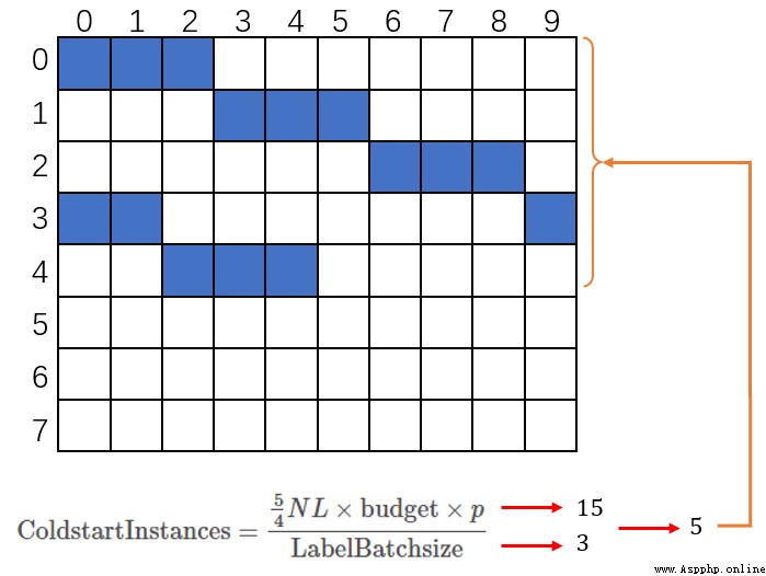
self.num_additional_queries = temp_num_additional_queriesThe batch calculation may be better understood by the formula ( Follow the parameter interpretation "\(p\)" The definition of ):\[\operatorname{ColdstartInstances} = \frac{\frac{5}{4}NL\times \text{budget} \times p}{\text{LabelBatchsize}} \tag{5}\] Why do cold start batches use "Instances" To express ? In fact, cold starts in code are not done batch by batch ( It's not strictly batch Training ), It's a one-time start . The code takes a batch of cold starts as one line , The number of tags per row should be equal , For example, our molecules have calculated 15 Number of tags , And limit a batch ( a line ) Check at most 3 A label , Then it will start cold 5 That's ok . this 5 The line is not divided into 5 Time training , Instead, it is integrated into a matrix and added to a training . In practice, our data sets are sorted by representativeness , Therefore, it often defaults to Top-ColdstartInstances Data cold start .
In addition, when selecting tags during cold start, try to select those tags with less query times , This is according to sparsity The principle of selection .
\[\operatorname{AdditionalQueries} = \frac{\frac{5}{4}NL\times \text{budget} \times (1-p)}{\text{InstanceBatchsize}} \tag{6}\] The second stage is the formal active learning stage , This part is genuine batch Training , The calculated number of additional queries is taken as the total number of batches , And execute such a total number of cycles , Each round robin query InstanceBatchsize Time , According to this query quantity, a new \(X^{\prime}\), \(Y^{\prime}\) Put in training , to update uncertainty And further query .
In this formula \(\frac{5}{4}NL\times \text{budget}\) In fact, it is a query upper limit estimated according to the data volume of the actual data set , In other words , This is the maximum total number of tags queried by experts , The second section introduces MASP The upper limit of the active learning process \(T\).
6.2.2 Rearrange data sets in a representative way
 self.compute_instance_representativeness(para_dc, 0)
temp_selected_array = self.representativeness_rank_array[0: temp_num_selected]
temp_dataset_select = self.dataset.select_data(temp_selected_array)
# Replace the training data with the selected part.
self.dataset = temp_dataset_select
self.network.dataset = temp_dataset_select
First, you need to rearrange the data through the representativeness of each data row , For the specific operation scheme, please refer to my This article Used in the Master Treelike Java programme (3.2~3.3), Of course, the plan is a little lengthy , Yes 100 Multiple lines , and Python Just a little 30 That's ok , Just don't get any better . Finally, the obtained representative sorting subscripts are used to guide the data set rearrangement , Get a sorted data set ( because MultiLabelAnn A copy of dataset, So there are dataset Also rearrange ).
 def compute_instance_representativeness(self, para_dc: float = 0.1, para_scheme: int = 0):
"""
Compute the representativeness of all instances.
:param para_dc: The dc ratio.
:return: An array.
"""
# Step 1. Calculate density using Gaussian kernel.
temp_dc_square = para_dc * para_dc
# The array length is n(n-1)/2.
temp_dist2 = torch.nn.functional.pdist(torch.from_numpy(self.dataset.data_matrix)).to(self.device)
# Convert to an n^2 matrix
temp_distances_matrix = scipy.spatial.distance.squareform(temp_dist2.cpu().numpy(), force='no', checks=True)
# Gaussian density.
temp_density_array = np.sum(np.exp(np.multiply(-temp_distances_matrix, temp_distances_matrix) / temp_dc_square),
axis=0)
# Step 2. Calculate distance to its master.
temp_distance_to_master_array = np.zeros(self.dataset.num_instances)
for i in range(self.dataset.num_instances):
temp_index = np.argwhere(temp_density_array > temp_density_array[i])
if temp_index.size > 0:
temp_distance_to_master_array[i] = np.min(temp_distances_matrix[i, temp_index])
# Step 3. Representativeness.
self.representativeness_array = temp_density_array * temp_distance_to_master_array
# Step 4. Sort instances according to representativeness.
self.representativeness_rank_array = np.argsort(self.representativeness_array)[::-1]
return self.representativeness_rank_array
In a word , Work out \(N\) The distance between data , Thus, the importance is obtained through the Gaussian optimization formula calculated according to the importance , Then each data point finds the nearest data point that is more important than itself, so as to obtain the independence and finally multiply it . This code should pay attention to the nature of matrix operations , Especially in the first 15 That's ok .
 # Step 2. Cold start stage.
# Can be revised to support the random label selection scheme. This is not the efficiency bottleneck.
for i in range(temp_cold_start_instances):
self.dataset.query_label_batch(i, self.dataset.get_scare_labels(para_label_batch))
print("two_stage_active_learn test 3")
self.bounded_train(para_pretrain_rounds, 100, para_enhancement_threshold)
self.cold_start_end_time = time.time()
In the cold start-up phase, it mainly passes through query_label_batch Complete the tag query , Create some new tag sets that are not missing . Then we use the cycle training to train this part of data .
 def get_scare_labels(self, para_length):
temp_indices = np.argsort(self.label_query_count_array)
result_array = np.zeros(para_length)
for i in range(para_length):
result_array[i] = temp_indices[i]
return result_array
In code get_scare_labels Method can return sparsity Satisfy Top-LabelBatchsize Tag set . The principle is not complicated , In fact, the label bucket is rearranged every time you select label_query_count_array, Select the first one with the lowest value LabelBatchsize Label subscripts . This variable is initially declared in MultiLabelData In the constructor of .
And determine the current \(i\) After the row and the label column array within the row, a stack of labels can be uniquely determined , After determining the label, you need to mark the label ( That is to say " Expert inquiry "), This operation is performed by dataset.query_label_batch Method .
 # Step 3. Active learning stage.
for i in range(temp_num_additional_queries):
print("Incremental training process: ", i, " out of ", temp_num_additional_queries)
temp_query_matrix = self.network.get_uncertain_label_batch(para_instance_batch)
for j in range(para_instance_batch):
self.dataset.query_label(int(temp_query_matrix[j][0]), int(temp_query_matrix[j][1]))
temp_input, temp_extended_label_matrix, temp_label_query_matrix = self.dataset.get_queried_instances()
for i in range(para_increment_rounds):
self.network.one_round_train(temp_input, temp_extended_label_matrix, temp_label_query_matrix)
self.multi_round_end_time = time.time()
self.bounded_train(200, 100, para_enhancement_threshold)
self.final_update_end_time = time.time()
The process of active learning is actually learning -> Get the maximum certainty, Perfect data set -> Study ->... The cycle of , Until the total number of cycles reaches the upper limit .
F1 I am introducing F1 when (4.3.3) And explain MultiLabelData Class to compress the array (5.4 Line 33, 47) Similar parameters have been made , Now a brief overview of its implementation :
 def my_test(self):
temp_test_start_time = time.time()
temp_input = torch.tensor(self.dataset.test_data_matrix[:], dtype=torch.float, device='cuda:0')
temp_predictions = self(temp_input)
temp_switch = temp_predictions[:,::2] < temp_predictions[:,1::2]
self.dataset.test_predicted_label_matrix = temp_switch.int()
self.dataset.test_predicted_proba_label_matrix = torch.exp(temp_predictions[:, 1::2]) / \
(torch.exp(temp_predictions[:, 1::2]) + torch.exp(temp_predictions[:, ::2]))
temp_test_end_time = time.time()
temp_my_testing_accuracy = self.dataset.compute_my_testing_accuracy()
temp_testing_f1 = self.dataset.compute_f1()
print("Test takes time: ", (temp_test_end_time - temp_test_start_time))
print("-------My test accuracy: ", temp_my_testing_accuracy, "-------")
print("-------My test f1: ", temp_testing_f1, "-------")
return temp_my_testing_accuracy, temp_testing_f1 def compute_f1(self):
"""
our F1
"""
temp_proba_matrix_to_vector = self.test_predicted_proba_label_matrix.reshape(-1).cpu().detach().numpy()
temp = np.argsort(-temp_proba_matrix_to_vector)
all_label_sort = self.test_label_matrix_to_vector[temp]
temp_y_F1 = np.zeros(temp.size)
all_TP = np.sum(self.test_label_matrix_to_vector == 1)
for i in range(temp.size):
TP = np.sum(all_label_sort[0:i+1] == 1)
P = TP / (i+1)
R = TP / all_TP
if (P+R)==0:
temp_y_F1[i] = 0
else:
temp_y_F1[i] = 2.0*P*R / (P+R)
return np.max(temp_y_F1)This part of the Union 4.3.3 Section to understand .
Peak-F1 Why on earth is it available ?
We are measuring Peak-F1 The label matrix is sorted , The aim is to ensure that most of the predictions are correct in the first place , This is the first practical 1 It can more match the positive tags we predicted . natural , If this is continuous 1 There is no inclusion 0, Successive 0 There is no inclusion 1, Then we can approach F1 Of best curve .
thus , Born out of best Curved two port softmax A threshold value must be found in the probability value \(\theta\), Greater than \(\theta\) The dual port prediction of is all correct after the label is positive , Less than \(\theta\) The predicted negative label is all correct . Rearrange the tag array with the predicted value again to form a perfect continuity 1 And continuity 0 A sort array of .
in other words \(\theta\) It has become a perfect watershed , There are no impurities around the watershed . such \(\theta\) The existence of can show that our network can 100% The prediction is correct . But in practice , No matter how good the multi label scheme is, it is impossible to find a way to achieve perfect segmentation \(\theta\), There are always impurities on the left and right , But the algorithm can find one as far as possible \(\theta\) Keep the impurities on the left and right as minimum as possible .
therefore Peak-F1 In essence, it describes that the multi label algorithm can find as perfect as possible \(\theta\) The ability of .
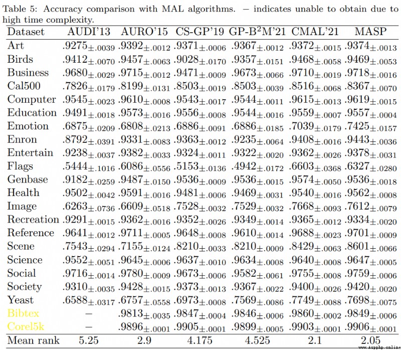
Finally, we will not show the relevant running results of the algorithm , This part can refer to the original paper . The thesis studies from supervision , Semi-supervised learning , Active learning Accuracy, as well as F1 result , The running time and other angles are compared with various multi label algorithms in parallel , The content is sufficiently detailed and substantial .
If the description in the article is biased, you are welcome to make corrections , Content bloggers about multi tags are also in the process of learning !