Catalog
One 、 Principle analysis
1.1 What does the image classification of computer vision mean ?
1.2 How to realize image classification ?
1.3Bag of features Algorithm and process
1) Extraction of image features
2) Training Dictionary
3) Image histogram generation
4) Training classifier
1.4TF-IDF
Two 、 Experimental process
2.1 The code analysis
2.2 Experimental process
2.3 experimental result
Image classification , That is, images are divided into different categories through different image contents ,
This technology was proposed in the late 1990s , It is named image classification based on image content (Content- Based ImageClassific- ation, CEIC) Algorithm concept ,
The content-based image classification technology does not need to label the semantic information of the image manually ,
Instead, the features contained in the image are extracted by computer , And process and analyze the characteristics , Get the classification results .
Common image features are Image color 、 texture 、 Grayscale and other information . In the process of image classification ,
The extracted features are not easy to be disturbed by random factors , Effective feature extraction can improve the accuracy of image classification .
After feature extraction , Select an appropriate algorithm to create the correlation between image types and visual features , Classify the images .
In the field of image classification , According to the image classification requirements , In general, it can be divided into Scene classification and There are two kinds of problems in target classification .
Scene classification can also be called event classification , Scene classification is right What the whole image represents Categorize the overall information , Or in the image A general description of the event that occurred .
Target classification ( Also known as object classification ) It's in the image The target that appears ( object ) To identify or classify .
Visual word bag model ( Bag-of-features ) It is a commonly used image representation method in the field of computer vision .
The visual word bag model comes from the word bag model (Bag-of-words), Word bag model was originally used in text classification , Representing a document as a feature vector . Its basic idea is to assume For a text , Ignore its word order and grammar 、 syntax , Just think of it as a collection of words , Each word in the text is independent . In short, each document is regarded as a bag ( Because it's full of words ,
So it's called word bag ,Bag of words That is why ) Look at the words in the bag , Classify them .
If there is a pig in the document 、 Horse 、 cattle 、 sheep 、 The valley 、 land 、 There are more words like tractor , And the bank 、 building 、 automobile 、 There are fewer words like Park , We tend to judge it as a A document depicting the countryside , Instead of describing the town .
Bag of Feature It also draws on this idea , Just in the image , What we draw out is no longer one by one word, It is Key features of the image Feature, So the researchers renamed it Bag of Feature.Bag of Feature The algorithm flow and classification in retrieval are almost the same , The only difference is , For the original BOF features , Histogram vector , We introduce TF_IDF A weight .
Image classification is a basic problem in the field of computer vision , Its purpose is to distinguish different types of images according to the semantic information of images , Achieve minimum classification error . The specific task requirement is to assign a label to the image from a given classification set . On the whole , For the single label image classification problem , It can be divided into image classification at the semantic level of cross species , Subclass fine-grained image classification , And instance level image classification . because VOC Data sets are data sets of different species categories , Therefore, this paper mainly studies and discusses the image classification task at the cross species semantic level .
Generally, there are the following technical difficulties in image classification :
(1) Change of perspective : The same object , The camera can show from many angles .
(2) Change in size : The visible size of an object usually changes .
(3) deformation : Many things are not in the same shape , There will be a big change . (4) Occlusion : The target object may be blocked . Sometimes only a small part of an object is visible .
(5) Light conditions : At the pixel level , The influence of light is very great .
(6) Background interference : Objects can get into the background , To make illegible .
(7) Intra class differences : There is a great difference in the shape of individuals of a class of objects , Like chairs . This kind of object has many different objects , Each has its own shape
Feature extraction and description are mainly about Representative and Highly differentiated Global or local features are extracted from the image , And describe these characteristics .
These characteristics are generally the comparison of the gap between categories Obvious features , It can be distinguished from other categories , secondly , These features also require Good stability , Can maximize the light 、 visual angle 、 scale 、 Keep stable when noise and various external factors change , Not affected by it . So even in very complex situations , The computer can also detect and recognize the object well through these stable features .
The simplest and most effective method of feature extraction is Regular grid method ,
This method uses uniform grid to divide the image , Thus, the local region features of the image are obtained .
Interest point detection is another effective feature extraction method , The basic idea of interest point detection is :
When artificially judging the category of an image , First, capture the overall contour features of the object , Then focus on where the object is significantly different from other objects , Finally, determine the category of the image . That is, through this object and other objects Distinguish between Salient features , Then judge the category of the image .
After extracting the features of the image , The next step is to use the feature descriptor to describe the extracted image features , The feature vector represented by the feature descriptor will generally be used as input data when processing the algorithm , therefore , If the descriptor has certain discrimination and distinguishability , Then the descriptor will play a great role in the later image processing .
among ,SIFT Descriptor is a classical and widely used descriptor in recent years .
SIFT Many feature points will be extracted from the picture , Each feature point is 128 Dimension vector , therefore , If there are enough pictures , We will extract a huge feature vector library .
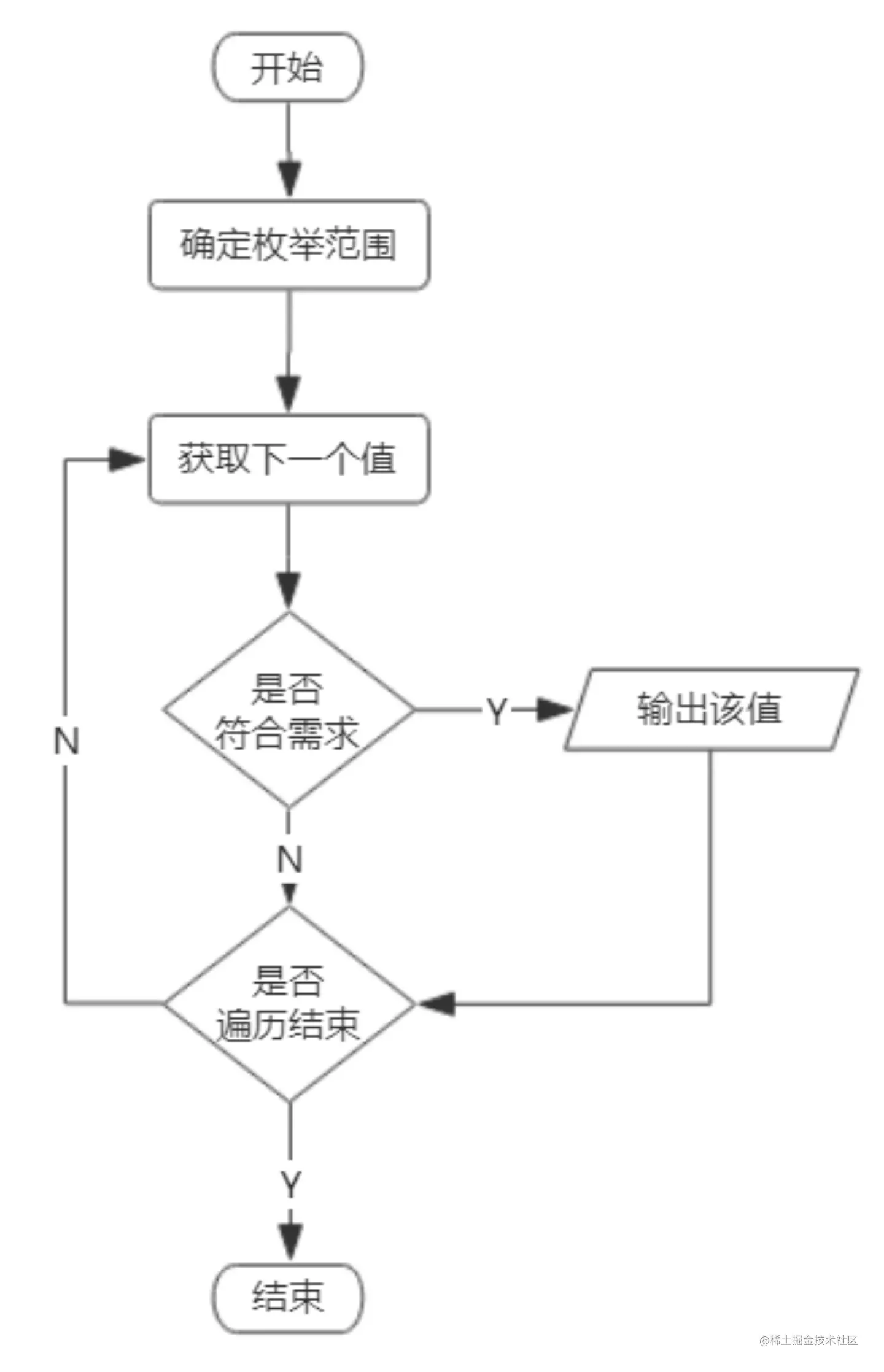
Finish extracting SIFT After the steps of the feature , utilize K-means The clustering algorithm will extract SIFT Feature clustering generates visual dictionary .
K-means Algorithm is a method to measure the similarity between samples , The algorithm sets the parameters to K, hold N An object is divided into K A cluster of , The similarity between clusters is high , The similarity between clusters is low . The cluster center has K individual , The visual dictionary is K. The process of building visual words is shown in the figure .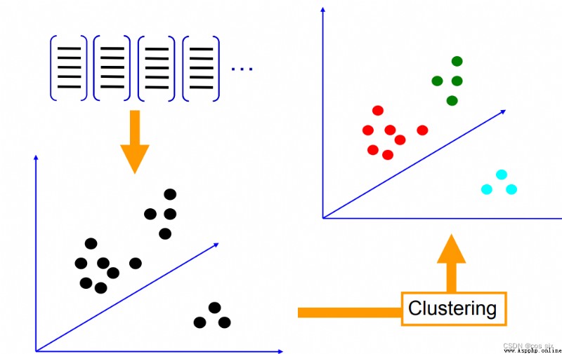
The words in the visual dictionary are used to represent the images to be classified . Calculate... In each image SIFT Feature here K The distance between two visual words ,
among The nearest visual word is this SIFT Visual words corresponding to features .
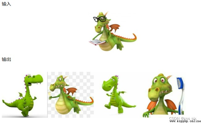
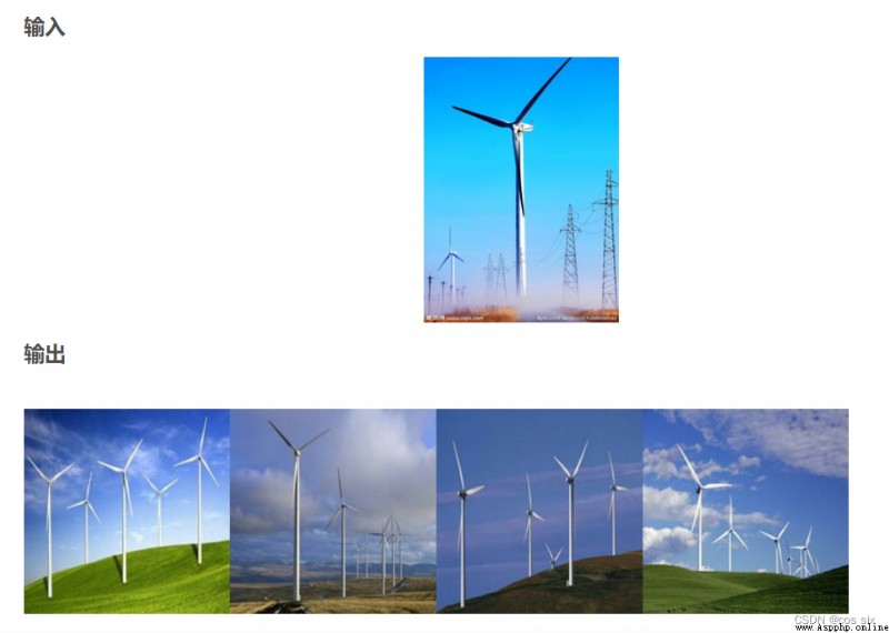
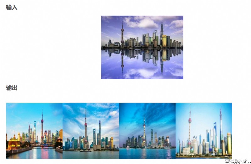
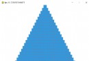
By counting the number of times each word appears in the image , Represent the image as a K One dimensional numerical vector ,
As shown in the figure , among K=4, Each image is described by histogram .
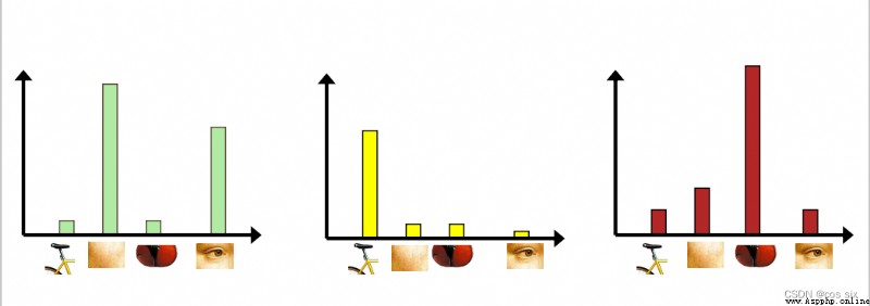
When we get the histogram vector of each picture , The rest of this step is the same as the previous steps .
It is nothing more than the vector of the database picture and the label of the picture , Train the classifier model . Then, for the pictures that need to be predicted , We still follow the above method , extract SIFT features , Then quantize the histogram vector according to the dictionary , The histogram vector is classified by classifier model . Of course , It can also be directly based on KNN The algorithm judges the similarity of histogram vector
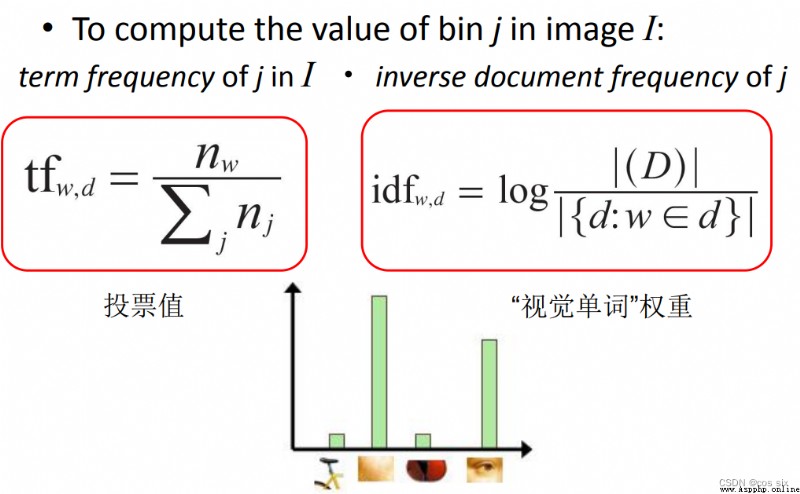
TF-IDF(Term frequency-Inverse document frequency) It's a statistical method , Used to evaluate the importance of feature words . according to TF-IDF The formula , The weight of feature words is the same as that in The frequency of occurrence in the corpus is related to , It is also related to the frequency of occurrence in the document . Conventional TF-IDF The formula is as follows
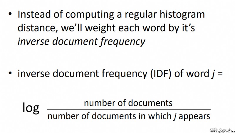
TF-IDF To evaluate the importance of a word to a document set or one of the documents in a corpus . The importance of a word increases in proportion to the number of times it appears in the document , But at the same time, it will decrease inversely with the frequency of its occurrence in the corpus . For now , If one Keywords only appear in very few web pages , Through it, we can Easy to lock the search target , its The weight should be Big . On the contrary, if a word appears in a large number of web pages , We see it still I'm not sure what I'm looking for , So it should Small .
Generate vocabulary :
# -*- coding: utf-8 -*-
import pickle
from PCV.imagesearch import vocabulary
from PCV.tools.imtools import get_imlist
from PCV.localdescriptors import sift
# Get image list
imlist = get_imlist('test/')
nbr_images = len(imlist)
# Get feature list
featlist = [imlist[i][:-3] + 'sift' for i in range(nbr_images)]
# Extract the image under the folder sift features
for i in range(nbr_images):
sift.process_image(imlist[i], featlist[i])
# Generating words
voc = vocabulary.Vocabulary('test77_test')
voc.train(featlist, 122, 10)
# Save vocabulary
# saving vocabulary
'''with open('D:/Program Files (x86)/QQdate/BagOfFeature/BagOfFeature/BOW/vocabulary.pkl', 'wb') as f:
pickle.dump(voc, f)'''
with open('C:/Users/86158/Desktop/ Computer vision experiment /Bag Of Feature/BOW/vocabulary.pkl', 'wb') as f:
pickle.dump(voc, f)
print('vocabulary is:', voc.name, voc.nbr_words)
Generate database :
import pickle
from PCV.imagesearch import vocabulary
from PCV.tools.imtools import get_imlist
from PCV.localdescriptors import sift
from PCV.imagesearch import imagesearch
from PCV.geometry import homography
from sqlite3 import dbapi2 as sqlite # Use sqlite As a database
# Get image list
imlist = get_imlist('test/')
nbr_images = len(imlist)
# Get feature list
featlist = [imlist[i][:-3]+'sift' for i in range(nbr_images)]
# load vocabulary
# Load vocabulary
with open('BOW/vocabulary.pkl', 'rb') as f:
voc = pickle.load(f)
# Create index
indx = imagesearch.Indexer('testImaAdd.db',voc) # stay Indexer Create tables in this class 、 Indexes , Write the image data to the database
indx.create_tables() # Create table
# go through all images, project features on vocabulary and insert
# Traverse all images , And project their features onto words
for i in range(nbr_images)[:888]:
locs,descr = sift.read_features_from_file(featlist[i])
indx.add_to_index(imlist[i],descr) # Use add_to_index Get an image with a feature descriptor , Project onto words
# Encode and store the word histogram of the image
# commit to database
# Commit to database
indx.db_commit()
con = sqlite.connect('testImaAdd.db')
print (con.execute('select count (filename) from imlist').fetchone())
print (con.execute('select * from imlist').fetchone())
Image search :
# -*- coding: utf-8 -*-
# The position information of image features is not included when using visual words to represent images
import pickle
from PCV.localdescriptors import sift
from PCV.imagesearch import imagesearch
from PCV.geometry import homography
from PCV.tools.imtools import get_imlist
# load image list and vocabulary
# Load image list
imlist = get_imlist('test/')
nbr_images = len(imlist)
# Load feature list
featlist = [imlist[i][:-3]+'sift' for i in range(nbr_images)]
# Load vocabulary
'''with open('E:/Python37_course/test7/first1000/vocabulary.pkl', 'rb') as f:
voc = pickle.load(f)'''
with open('BOW/vocabulary.pkl', 'rb') as f:
voc = pickle.load(f)
src = imagesearch.Searcher('testImaAdd.db',voc)# Searcher Class reads the word histogram of the image and executes the query
# index of query image and number of results to return
# Query the image index and the number of images returned by the query
q_ind = 0
nbr_results = 130
# regular query
# Regular query ( Sort the results by Euclidean distance )
res_reg = [w[1] for w in src.query(imlist[q_ind])[:nbr_results]] # Result of query
print ('top matches (regular):', res_reg)
# load image features for query image
# Load query image features for matching
q_locs,q_descr = sift.read_features_from_file(featlist[q_ind])
fp = homography.make_homog(q_locs[:,:2].T)
# RANSAC model for homography fitting
# Fitting with homography to establish RANSAC Model
model = homography.RansacModel()
rank = {}
# load image features for result
# Load features of candidate images
for ndx in res_reg[1:]:
try:
locs,descr = sift.read_features_from_file(featlist[ndx])
except:
continue
#locs,descr = sift.read_features_from_file(featlist[ndx]) # because 'ndx' is a rowid of the DB that starts at 1
# get matches
matches = sift.match(q_descr,descr)
ind = matches.nonzero()[0]
ind2 = matches[ind]
tp = homography.make_homog(locs[:,:2].T)
# compute homography, count inliers. if not enough matches return empty list
# Calculate the homography matrix
try:
H,inliers = homography.H_from_ransac(fp[:,ind],tp[:,ind2],model,match_theshold=4)
except:
inliers = []
# store inlier count
rank[ndx] = len(inliers)
# sort dictionary to get the most inliers first
# Sort the dictionary , You can get the query results after rearrangement
sorted_rank = sorted(rank.items(), key=lambda t: t[1], reverse=True)
res_geom = [res_reg[0]]+[s[0] for s in sorted_rank]
print ('top matches (homography):', res_geom)
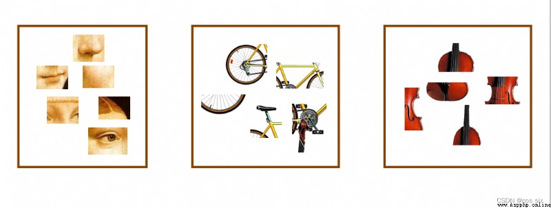
# Show query results
imagesearch.plot_results(src,res_reg[:6]) # Regular query
imagesearch.plot_results(src,res_geom[:6]) # The result of the rearrangement
Data sets :
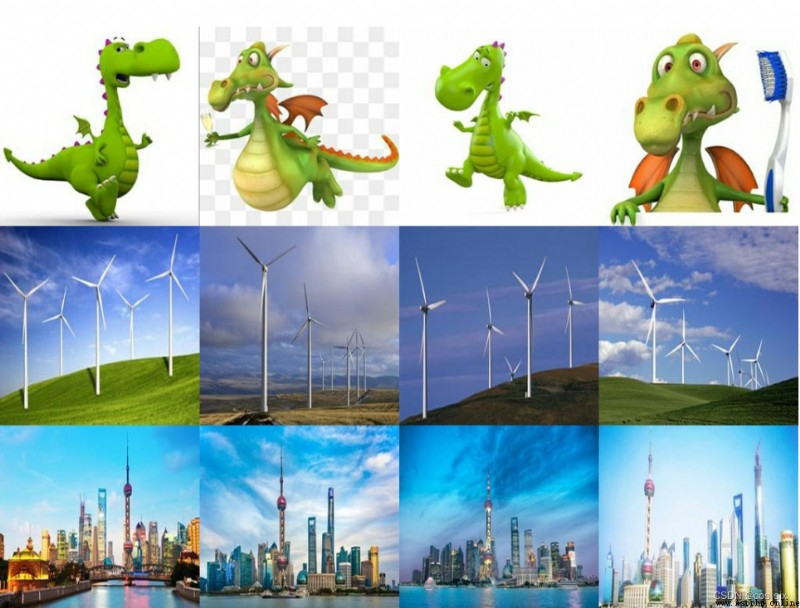
Test set :