正則化-線性回歸及logistic回歸的應用與python實現

• 過擬合問題 overfitting
• • 問題識別
  • 過擬合問題解決
• 代價函數 cost function
• 線性回歸的正則化
• logistic回歸的正則化
• 代碼實現+可視化

過擬合問題 overfitting

問題識別

• 欠擬合（underfitting ) 或 高偏差（high bias），擬合效果差
• 恰好擬合（just right）
• 過擬合（overfiiting）或 高方差（high variance 函數太過於龐大、變量太多），泛化能力（generalization ability）差
  
  

過擬合問題解決

• 減少特征變量個數
• 正則化（regularizition）。保留所有特征變量，但減小特征變量量級或降低變量在假設方程中的參數大小；從而使得每個特征變量對預測結果僅僅貢獻部分作用。
  

代價函數 cost function

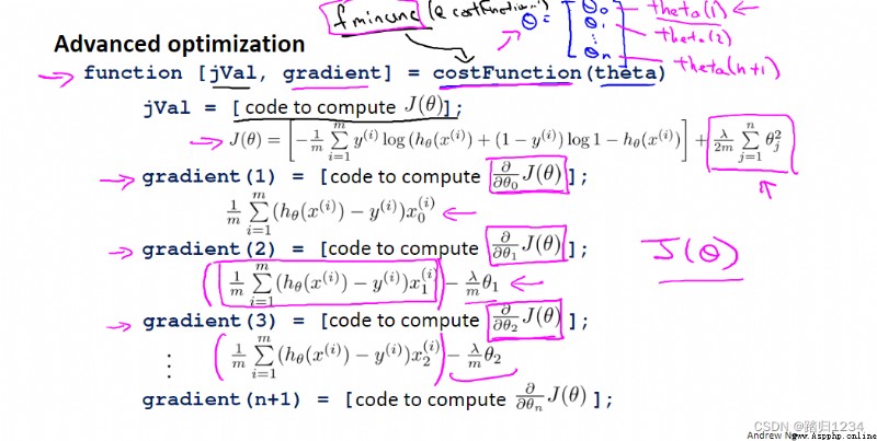
目標：介紹正則化（regularizition）如何應用，並寫出相應的代價函數。
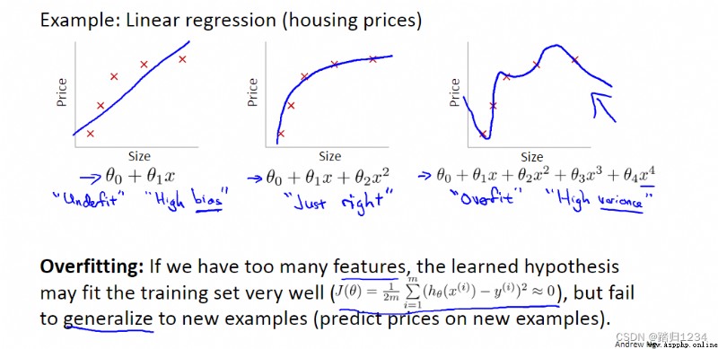
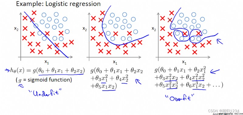
比如，在代價函數中加入 θ 3 、 θ 4 \theta_3 、\theta_4 θ3​、θ4​的懲罰項，使得它們接近於0，最終的假設模型中 x 3 、 x 4 x^3、x^4 x3、x4的系數很,小，從而假設模型近似於二次函數。

如果參數值較小，那麼參數值較小意味著一個更加簡單的假設模型（hypothesis）。一般來說，這會使得最終得到的函數更加平滑、更加簡單，也不容易出現過擬合問題。
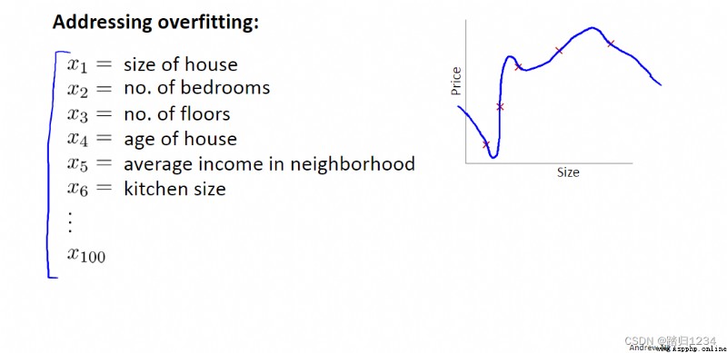
在實際應用中，因為不知道哪個特征變量屬於高階項，所以修改代價函數，直接縮小所有的參數，即 J ( θ ) J(\theta) J(θ)。值得注意的是，代價函數中沒有給 θ 0 \theta_0 θ0​增加懲罰項，這是約定俗稱的一種做法，實際上無論是否給它加入懲罰項對結果的影響都不大。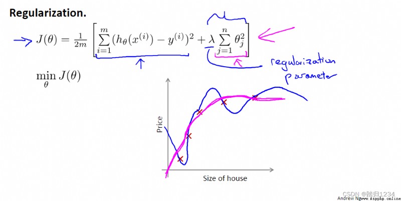

正則化代價函數 J ( θ ） J(\theta） J(θ）（regularized cost function ，正則化的優化目標 regularized optimization objective）中最右邊的求和項即正則化項（regularization term）， λ \lambda λ為正則化參數（regularization parameter）。 λ \lambda λ的作用即為控制不同目標間的取捨，目標一：更好得擬合數據集；目標二：保持參數盡可能小。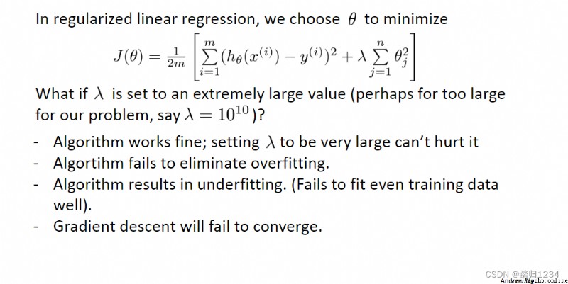


λ \lambda λ越大，各個 θ \theta θ越接近0，相當於把假設模型中的各個特征變量都忽略，從而導致擬合直線幾乎變成一條平行的直線，導致擬合效果不好。因此需要合理選擇正則化參數 λ \lambda λ的值。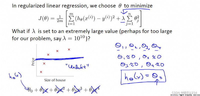

線性回歸的正則化

目標：正則化在線性回歸方程中的應用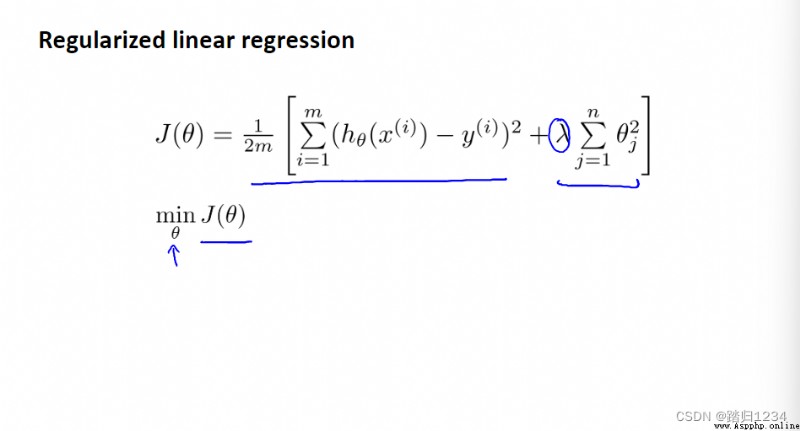

線性回歸梯度下降時，參數 θ \theta θ變化如下。
θ j : = θ j ( 1 − α λ m ) − α 1 m ∑ i = 0 m ( h θ ( x ( i ) ) − y ( i ) ) x j ( i ) \theta_j := \theta_j(1-\alpha\frac \lambda m)-\alpha \frac 1m \sum_{i=0}^m(h_\theta (x^{(i)})-y^{(i)})x_j^{(i)} θj​:=θj​(1−αmλ​)−αm1​∑i=0m​(hθ​(x(i))−y(i))xj(i)​
其中， 1 − α λ m 1-\alpha\frac \lambda m 1−αmλ​通常是比1略微小的數。
因此，直觀來說，正則化即每次把參數縮小一點點。從數學上來說，所做的還是對代價函數 J θ J\theta Jθ進行梯度下降。
注意， θ 0 \theta_0 θ0​不用添加 λ m θ 0 \frac \lambda m \theta_0 mλ​θ0​。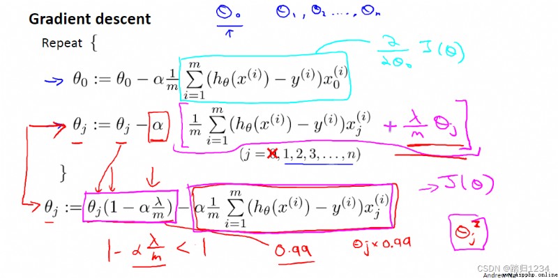

梯度下降只是擬合線性回歸模型的一種方法，下面展示另一種方法——正規方程（normal equation）。
設計一個m*(n+1)維 矩陣X，它的每一行都代表一個單獨的訓練樣本。建立一個m維向量y，包含訓練集裡的所有標簽。
則，全局最小值的參數 θ \theta θ 如下：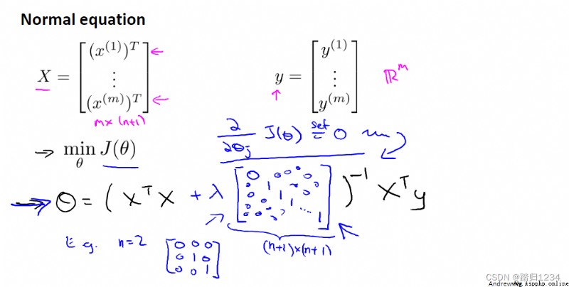

對於一般的線性方程，當m小於等於n時，矩陣 X T X X^TX XTX不可逆，正規方程不可用。
但對於正則化後的方程，可以保證 X T X + λ [ 0 0 ⋯ 0 0 1 ⋯ 0 ⋮ ⋮ ⋱ ⋮ 0 0 ⋯ 1 ] X^TX+\lambda\begin{bmatrix} 0&0&{ \cdots }&0\\ 0&1&{ \cdots }&0\\ { \vdots }&{ \vdots }&{ \ddots }&{ \vdots }\\ 0&0&{ \cdots }&1 \end{bmatrix} XTX+λ⎣⎡​00⋮0​01⋮0​⋯⋯⋱⋯​00⋮1​⎦⎤​ 為非奇異矩陣，即一定可逆。
因此正則化還可以解決正規方程中的不可逆問題。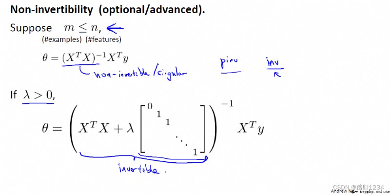

logistic回歸的正則化

目標：了解正則化如何應用到logistic回歸函數。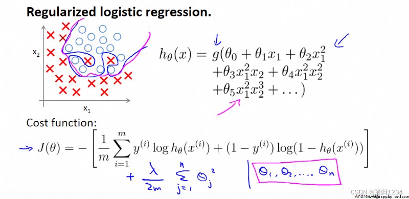

與線性回歸類似，也是在 θ j \theta_j θj​中加入 λ m θ j \frac \lambda m \theta_j mλ​θj​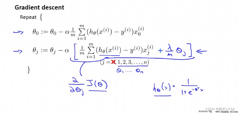

代碼實現+可視化

正則化邏輯回歸 python代碼實現

"logistic regression"
import pandas as pd
import numpy as np
import matplotlib.pyplot as plt
import seaborn as sns
from sklearn.model_selection import train_test_split
from sklearn.preprocessing import StandardScaler#標准化
from sklearn.metrics import confusion_matrix,roc_curve,auc,classification_report #分類度量方法
class logisticRegressionGradientDescent:
""" 邏輯回歸，采用批量梯度下降，交叉熵損失函數 """
def __init__(self,dataset,attribute_list,aplha,mylambda):
""" 類初始化 :param dataset:數據集 :param attribute_list:特征列表 :param aplha:學習率 :param mylambda:正則化參數 """
self.alpha=aplha
self.attr_list =attribute_list[:-1]#特征值
self.target_lable=attribute_list[-1]#目標列名（取最後一列）
#數據標准化
self.X= StandardScaler().fit_transform(dataset.iloc[:,:-1])
#對目標值進行編碼
self.y,self.class_lables = self.target_encode(dataset.iloc[:,-1])
#劃分數據集,分層抽樣(stratify 按照列標y) random_state隨機種子，防止每次運行結果重現
self.x_train,self.x_test,self.y_train,self.y_test=\
train_test_split(self.X,self.y,train_size=0.8,random_state=1,stratify=self.y)
self.n,self.k=self.x_train.shape #訓練數據樣本量，特征變量個數
self.cross_entropy_cost = []#每次訓練交叉熵的平均值
self.bdg_weight= dict()#每次訓練權重更新
self.mylambda=mylambda#正則化參數
@staticmethod
def sigmoid(y_preval):
''' 激活函數 :param y_preval: 樣本值乘以權重系數後的值，數組 :return: '''
return 1/(1+np.exp(-y_preval))
@staticmethod
def target_encode(target):
""" 靜態方法，不用self,標記 @staticmethod 二分類類別編碼為0,1 :param self: :param target: 類別列表 :return: """
class_lables=target.unique()# 獲取不同類別值
if len(class_lables)>2:
print("此邏輯回歸只是限於二分類，請選擇多分類算法")
exit(0)
if(class_lables.max()==1 and class_lables.min()==0):
return target.tolist(),class_lables
else:
#編碼，采用列表推導式
target_y = [0 if y == class_lables[0] else 1 for y in target]
return target_y,class_lables
def logistic_regression_model_train(self,max_lop,threshold):
''' 邏輯回歸訓練函數，采用批量梯度下降法，交叉熵損失函數 :param max_lop: 最大訓練次數 :param threshold:退出訓練阈值 :return: '''
np.random.seed(101)#設置隨機種子，避免每次都一樣
weight =np.random.random(self.k)/100 #隨機化權重 權重數同特征變量數 random模塊的random函數
weight_old =weight
for j in range(self.k):
self.bdg_weight[str(j)]=[]
for loop in range(max_lop):
self.alpha*=0.95#衰減指數慢慢減少
y_hat = self.sigmoid(self.x_train.dot(weight.T))#激活函數·，預測屬於某一類別的概率（0,1） 求x乘以權重 矩陣計算
dw= ((y_hat-self.y_train)*self.x_train.T).mean(axis=1)#權值更新 對所有的列求均值 結果等同於(self.x_train.T*(y_hat-self.y_train)).mean(axis=1)
weight=(1-self.alpha*mylambda/len(y_hat))*weight-self.alpha*dw #權值更新
#weight=weight-self.alpha*dw #權值更新 未正則化
for j in range(self.k):
self.bdg_weight[str(j)].append(weight[j])
#交叉熵損失均值 1e-10是因為防止log後取值太小對結果產生影響
ce_loss =-(np.array(self.y_train)*np.log(y_hat+1e-10)+
(1-np.array(self.y_train))*np.log(1-y_hat+1e-10)).mean()+1/2*mylambda*np.power(weight, 2).sum()/len(y_hat)
# ce_loss =-(np.array(self.y_train)*np.log(y_hat+1e-10)+
# (1-np.array(self.y_train))*np.log(1-y_hat+1e-10)).mean()#未正則化
self.cross_entropy_cost.append(ce_loss)
#退出條件，避免過擬合，提前停止訓練
if(len(self.cross_entropy_cost)>2):
if np.abs(self.cross_entropy_cost[-1]-self.cross_entropy_cost[-2])>threshold:
break
elif np.abs(weight-weight_old).all()<threshold:
break
else:
weight_old=weight
# #畫圖
# plt.plot(self.cross_entropy_cost)
# plt.show()
return weight
def plt_cost(self):
""" 繪制交叉熵損失下降曲線 :return: """
plt.plot(self.cross_entropy_cost)
plt.xlabel("Training times")
plt.ylabel("Cross entropy cost")
plt.title("Decline curve of loss function in Logistic regression")
# plt.show()
def plt_weight(self):
""" 繪制權重更新曲線 :return: """
for k in range(self.k):
plt.plot(self.bdg_weight[str(k)],label=self.attr_list[k])
plt.legend()
plt.xlabel("Training times")
plt.ylabel("Weight")
plt.title("Logistic regression weight coefficient update curve")
def predict(self,weight):
""" 測試樣本預測類別，並根據概率進行類別編碼 :param weight:訓練最終權重 :return: """
y_pred =[]#預測類別
y_score =self.sigmoid(self.x_test.dot(weight.T))
threshold =0.5 # 類別不平衡問題需要考慮阈值，待解決
for y in y_score:
if y<threshold:
y_pred.append(0)
elif y>= threshold:
y_pred.append(1)
cm= confusion_matrix(self.y_test,y_pred)
acc= np.sum(np.diag(cm))/len(y_pred) #預測精度
return y_pred,cm,acc,y_score
def plt_confusion_matrix(self,cm,acc):
""" 繪制混淆矩陣 :param cm: 混淆矩陣 :param acc: 預測精度 :return: """
cm =pd.DataFrame(cm,columns=self.class_lables,index=self.class_lables)
sns.heatmap(cm,annot=True,cbar=False,fmt='d')#繪制熱圖
plt.xlabel("Predict")
plt.ylabel("True")
plt.title("Confusion matrix and accuracy =%.2f%%" %(acc*100))#%%表示直接輸出一個%
def plt_roc_auc(self,y_score):
""" 繪制ROC曲線，並計算AUC :param y_score: 預測樣本預測評分 :return: """
false_positive_rate,true_positive_rate,_ =roc_curve(self.y_test,y_score)
roc_auc=auc(false_positive_rate,true_positive_rate)
plt.plot(false_positive_rate,true_positive_rate,"b",label="AUC=%.2f" % roc_auc)
plt.legend(loc="lower right")
plt.plot([0,1],[0,1],"r--")
plt.xlabel("False_positive_rate")
plt.ylabel("True_positive_rate")
plt.title("Logistic Regression of Binary Classification ROC Curve and AUC")
if __name__=='__main__':
url="../datasets/Mtrain_set.csv"#數據集路徑
data=pd.read_csv(url).dropna().iloc[:,1:]
attribute_list =data.columns#列名列表 list列表，沒有loc屬性
alpha =0.8
mylambda=1000
#print(attribute_list)
lrgd=logisticRegressionGradientDescent(data,attribute_list,alpha,mylambda)#正則化處理
# lrgd=logisticRegressionGradientDescent(data,attribute_list,alpha)#沒有正則化
weight=lrgd.logistic_regression_model_train(1000,1e-8)
print("正則化邏輯回歸，采用批量梯度下降法訓練，最終特征變量系數：")
for i in range(lrgd.k):
print(" %-10s %.15f" % (lrgd.attr_list[i],weight[i]))
y_pred,cm,acc,y_score =lrgd.predict(weight)
#繪圖
plt.figure(figsize=(12,10))
plt.subplot(221)#表示將整個圖像窗口分為2行2列, 當前位置為1.
lrgd.plt_cost()
plt.subplot(222)
lrgd.plt_weight()
plt.subplot(223)
lrgd.plt_confusion_matrix(cm,acc)
plt.subplot(224)
lrgd.plt_roc_auc(y_score)
plt.show()
#還可以再打印出一個分類報告

運行結果
數據擬合效果欠佳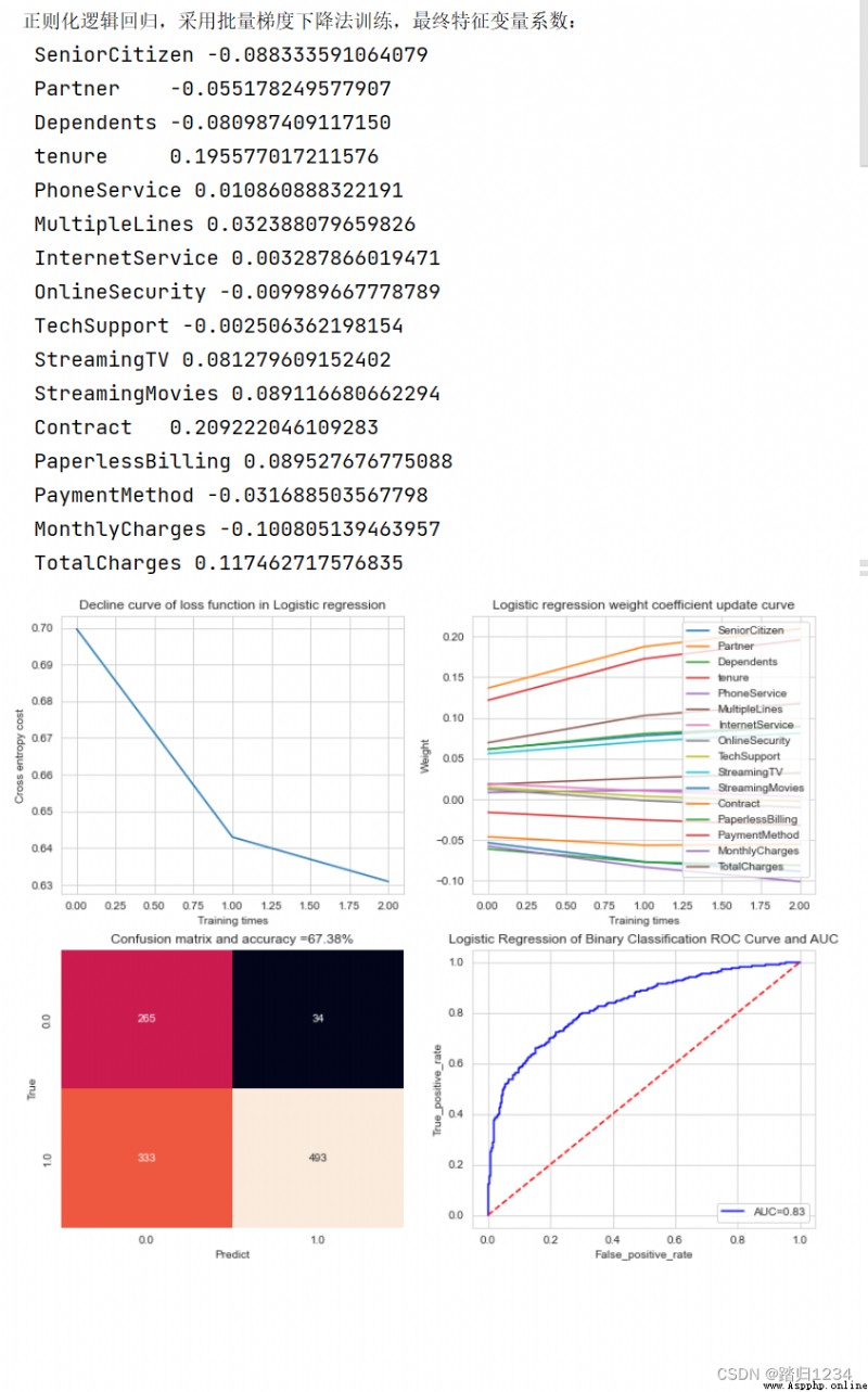

參考資料
網易版 吳恩達機器學習
2021機器學習（西瓜書+李航統計學習方法）實踐部分 + Python