numpy The general function of pandas The object operation :
In [190]: frame = pd.DataFrame(np.random.randn(4, 3), columns=list('bde'),
.....: index=['Utah', 'Ohio', 'Texas', 'Oregon'])
In [191]: frame
Out[191]:
b d e
Utah -0.204708 0.478943 -0.519439
Ohio -0.555730 1.965781 1.393406
Texas 0.092908 0.281746 0.769023
Oregon 1.246435 1.007189 -1.296221
In [192]: np.abs(frame)
Out[192]:
b d e
Utah 0.204708 0.478943 0.519439
Ohio 0.555730 1.965781 1.393406
Texas 0.092908 0.281746 0.769023
Oregon 1.246435 1.007189 1.296221
Another common operation is , Apply the function to a one-dimensional array formed by columns or rows .DataFrame Of apply Method to achieve this function :
In [193]: f = lambda x: x.max() - x.min()
In [194]: frame.apply(f)
Out[194]:
b 1.802165
d 1.684034
e 2.689627
dtype: float64
Functions here f, Calculated a Series The difference between the maximum and minimum of , stay frame Each column of is executed once . The result is a Series, Use frame As an index .
If you deliver axis='columns' To apply, This function will execute on each line :
In [195]: frame.apply(f, axis='columns')
Out[195]:
Utah 0.998382
Ohio 2.521511
Texas 0.676115
Oregon 2.542656
dtype: float64
Pass on to apply The function of does not have to return a scalar , You can also return a combination of multiple values Series:
In [196]: def f(x):
.....: return pd.Series([x.min(), x.max()], index=['min', 'max'])
In [197]: frame.apply(f)
Out[197]:
b d e
min -0.555730 0.281746 -1.296221
max 1.246435 1.965781 1.393406
Sorting has always been an indispensable part of data . To sort a row or column index , have access to sort_index Method , It will return a new object that has been sorted :
In [201]: obj = pd.Series(range(4), index=['d', 'a', 'b', 'c'])
In [202]: obj.sort_index()
Out[202]:
a 1
b 2
c 3
d 0
dtype: int64
It's about Series, Of course for DataFrame There are similar operations :
In [203]: frame = pd.DataFrame(np.arange(8).reshape((2, 4)),
.....: index=['three', 'one'],
.....: columns=['d', 'a', 'b', 'c'])
In [204]: frame.sort_index()
Out[204]:
d a b c
one 4 5 6 7
three 0 1 2 3
In [205]: frame.sort_index(axis=1)
Out[205]:
a b c d
three 1 2 3 0
one 5 6 7 4
Data is sorted in ascending order by default , But it can also be sorted in descending order :
In [206]: frame.sort_index(axis=1, ascending=False)
Out[206]:
d c b a
three 0 3 2 1
one 4 7 6 5
To pair by value Series Sort , It can be used sort_values Method :
In [207]: obj = pd.Series([4, 7, -3, 2])
In [208]: obj.sort_values()
Out[208]:
2 -3
3 2
0 4
1 7
dtype: int64
When sorting a DataFrame when , You may want to sort based on the values in one or more columns . Pass the name of one or more columns to sort_values Of by Option to achieve this :
In [211]: frame = pd.DataFrame({'b': [4, 7, -3, 2], 'a': [0, 1, 0, 1]})
In [212]: frame
Out[212]:
a b
0 0 4
1 1 7
2 0 -3
3 1 2
In [213]: frame.sort_values(by='b')
Out[213]:
a b
2 0 -3
3 1 2
0 0 4
1 1 7
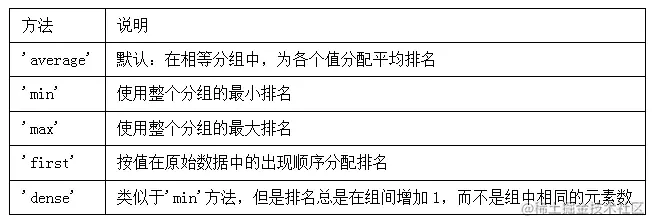
Finish sorting , Next is the ranking , The so-called ranking refers to the array from 1 The operation of assigning ranking to the total number of valid data points .Series and DataFrame Of rank Method is a functional method to achieve ranking . By default ,rank Break the tie by assigning an average ranking to each group :
In [215]: obj = pd.Series([7, -5, 7, 4, 2, 0, 4])
In [216]: obj.rank()
Out[216]:
0 6.5
1 1.0
2 6.5
3 4.5
4 3.0
5 2.0
6 4.5
dtype: float64
In short, it is to size the data . Small from 1 Start , The big one is behind , In case of repetition, take the average value . You can also rank according to the order in which the values appear in the original data :
In [217]: obj.rank(method='first')
Out[217]:
0 6.0
1 1.0
2 7.0
3 4.0
4 3.0
5 2.0
6 5.0
dtype: float64
here , entry 0 and 2 Average ranking is not used 6.5, They are set to 6 and 7, Because the labels in the data 0 Located on the label 2 In front of .
Of course, you can also arrange them in reverse order , It can also be in DataFrame Use in :
In [219]: frame = pd.DataFrame({'b': [4.3, 7, -3, 2], 'a': [0, 1, 0, 1],
.....: 'c': [-2, 5, 8, -2.5]})
In [220]: frame
Out[220]:
a b c
0 0 4.3 -2.0
1 1 7.0 5.0
2 0 -3.0 8.0
3 1 2.0 -2.5
In [221]: frame.rank(axis='columns')
Out[221]:
a b c
0 2.0 3.0 1.0
1 1.0 3.0 2.0
2 2.0 1.0 3.0
3 2.0 3.0 1.0
chart 5-3 Shows the occurrence of horizontal level in sorting ( The values are the same ) How to distinguish the priority method in the case of .
What should we do when our labels are duplicated ? Let's take a look at the following simple with duplicate index values Series:
In [222]: obj = pd.Series(range(5), index=['a', 'a', 'b', 'b', 'c'])
In [223]: obj
Out[223]:
a 0
a 1
b 2
b 3
c 4
dtype: int64
Indexed is_unique Property can tell you whether its value is unique :
In [224]: obj.index.is_unique
Out[224]: False
For indexes with duplicate values , The behavior of data selection will be somewhat different . If an index corresponds to multiple values , Returns a Series; Corresponding to a single value , Returns a scalar value :
In [225]: obj['a']
Out[225]:
a 0
a 1
dtype: int64
In [226]: obj['c']
Out[226]: 4
This will complicate the code , Because the output type of the index will change according to whether the label is repeated . Yes DataFrame The same is true when indexing rows of . Therefore, we try to avoid duplicate axis indexes in use .
pandas Have a set of commonly used mathematical and statistical methods . Most of them belong to the classification of reduction or summary statistics . These methods range from DataFrame Extract one from the row or column of Series Or a single value of a series of values ( For example, statistics and or average value ). And Numpy Compared with similar methods in the array , They have built-in functions for processing loss values . For a small DataFrame:
In [230]: df = pd.DataFrame([[1.4, np.nan], [7.1, -4.5],
.....: [np.nan, np.nan], [0.75, -1.3]],
.....: index=['a', 'b', 'c', 'd'],
.....: columns=['one', 'two'])
In [231]: df
Out[231]:
one two
a 1.40 NaN
b 7.10 -4.5
c NaN NaN
d 0.75 -1.3
call DataFrame Of sum Method will return a that contains the sum of the columns Series:
In [232]: df.sum()
Out[232]:
one 9.25
two -5.80
dtype: float64
Pass in axis='columns' or axis=1 Will sum by line :
In [233]: df.sum(axis=1)
Out[233]:
a 1.40
b 2.60
c NaN
d -0.55
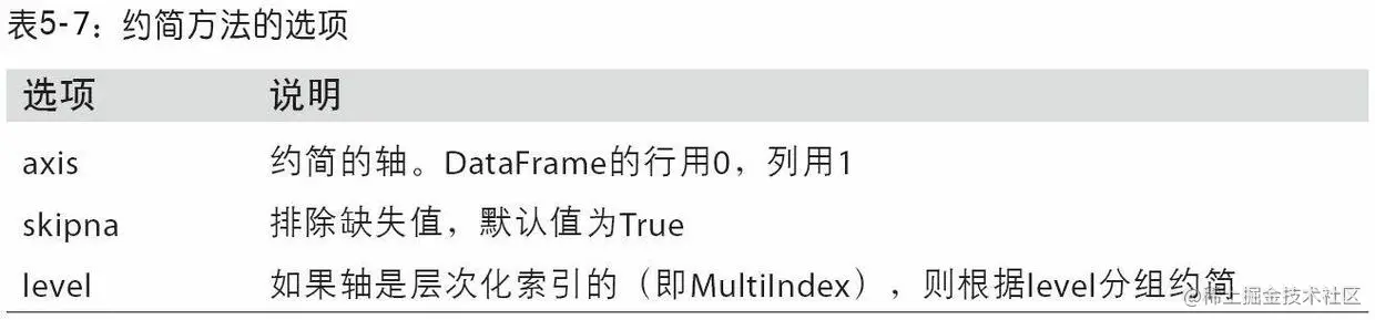
NA Values are automatically excluded , Unless the whole slice ( This refers to rows or columns ) All are NA. adopt skipna Option to disable this feature :
In [234]: df.mean(axis='columns', skipna=False)
Out[234]:
a NaN
b 1.300
c NaN
d -0.275
dtype: float64
The figure below 5-4 The common parameters of reduction methods are listed
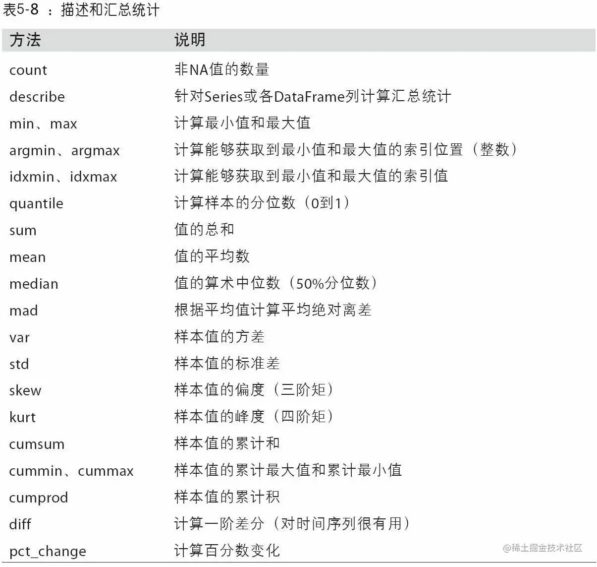
There are many other methods that will not be shown one by one , The figure below 5-5 It shows a list of methods related to summary statistics .
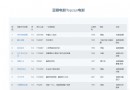
Summary statistics , For example, there is correlation and covariance , These are calculated by many parameters . Let's take a look at an actual data example , They come from Yahoo!Finance The stock price and trading volume of , If you need the data set here, you can ask me for a private message :
In [240]: price = pd.read_pickle('examples/yahoo_price.pkl')
In [241]: volume = pd.read_pickle('examples/yahoo_volume.pkl')
In [242]: returns = price.pct_change()
In [243]: returns.tail()
Out[243]:
AAPL GOOG IBM MSFT
Date
2016-10-17 -0.000680 0.001837 0.002072 -0.003483
2016-10-18 -0.000681 0.019616 -0.026168 0.007690
2016-10-19 -0.002979 0.007846 0.003583 -0.002255
2016-10-20 -0.000512 -0.005652 0.001719 -0.004867
2016-10-21 -0.003930 0.003011 -0.012474 0.042096
The percentage of data price is calculated here .
Series Of corr Method is used to calculate two Series Overlapping in 、 Not NA Of 、 Correlation coefficient of index aligned values . A similar ,cov Used to calculate covariance :
In [244]: returns['MSFT'].corr(returns['IBM'])
Out[244]: 0.49976361144151144
In [245]: returns['MSFT'].cov(returns['IBM'])
Out[245]: 8.8706554797035462e-05
because MSTF It's a reasonable Python attribute , We can also select columns in a more concise syntax :
In [246]: returns.MSFT.corr(returns.IBM)
Out[246]: 0.49976361144151144
On the other hand ,DataFrame Of corr and cov Method will DataFrame Return the complete correlation coefficient or covariance matrix respectively :
In [247]: returns.corr()
Out[247]:
AAPL GOOG IBM MSFT
AAPL 1.000000 0.407919 0.386817 0.389695
GOOG 0.407919 1.000000 0.405099 0.465919
IBM 0.386817 0.405099 1.000000 0.499764
MSFT 0.389695 0.465919 0.499764 1.000000
In [248]: returns.cov()
Out[248]:
AAPL GOOG IBM MSFT
AAPL 0.000277 0.000107 0.000078 0.000095
GOOG 0.000107 0.000251 0.000078 0.000108
IBM 0.000078 0.000078 0.000146 0.000089
MSFT 0.000095 0.000108 0.000089 0.000215
utilize DataFrame Of corrwith Method , You can calculate its column or row with another Series or DataFrame The correlation coefficient between . Pass in a Series A correlation coefficient value will be returned Series( Calculate for each column ):
In [249]: returns.corrwith(returns.IBM)
Out[249]:
AAPL 0.386817
GOOG 0.405099
IBM 1.000000
MSFT 0.499764
dtype: float64
Pass in a DataFrame The correlation coefficient paired by column name is calculated . here , I calculate the correlation coefficient between the percentage change and the trading volume :
In [250]: returns.corrwith(volume)
Out[250]:
AAPL -0.075565
GOOG -0.007067
IBM -0.204849
MSFT -0.092950
dtype: float64
Pass in axis='columns' It can be calculated by line . in any case , Before calculating the correlation coefficient , All data items will be aligned by labels .
Another kind of method is from one dimension Series Extract information from the contained values . For simplicity , Here's an example :
In [251]: obj = pd.Series(['c', 'a', 'd', 'a', 'a', 'b', 'b', 'c', 'c'])
The first function is unique, It can get Series Array of unique values in :
In [252]: uniques = obj.unique()
In [253]: uniques
Out[253]: array(['c', 'a', 'd', 'b'], dtype=object)
The only value returned is unordered , If necessary , You can sort the results again (uniques.sort()). alike ,value_counts Used to calculate a Series The frequency of occurrence of each value in :
In [254]: obj.value_counts()
Out[254]:
c 3
a 3
b 2
d 1
dtype: int64
For ease of viewing , result Series It is arranged in descending order of value frequency .value_counts It is also a top class pandas Method , Can be used with any array or sequence :
In [255]: pd.value_counts(obj.values, sort=False)
Out[255]:
a 3
b 2
c 3
d 1
dtype: int64
isin Used to determine the membership of a vectorized set , Can be used to filter Series Medium or DataFrame Subset of data in column :
In [256]: obj
Out[256]:
0 c
1 a
2 d
3 a
4 a
5 b
6 b
7 c
8 c
dtype: object
In [257]: mask = obj.isin(['b', 'c'])
In [258]: mask
Out[258]:
0 True
1 False
2 False
3 False
4 False
5 True
6 True
7 True
8 True
dtype: bool
In [259]: obj[mask]
Out[259]:
0 c
5 b
6 b
7 c
8 c
dtype: object
And isin similarly Index.get_indexer Method , It can give you an index array , From an array that may contain duplicate values to another array of different values :
In [260]: to_match = pd.Series(['c', 'a', 'b', 'b', 'c', 'a'])
In [261]: unique_vals = pd.Series(['c', 'b', 'a'])
In [262]: pd.Index(unique_vals).get_indexer(to_match)
Out[262]: array([0, 2, 1, 1, 0, 2])
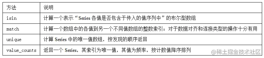
chart 5-6 Some reference information of these methods is given .
This chapter is about this , In the next chapter , We will discuss the use of pandas Read ( Or load ) And tools for writing data sets . after , We will look more deeply into the use of pandas Data cleaning 、 Be regular 、 Analysis and visualization tools .