說明:這是一個機器學習實戰項目(附帶數據+代碼+文檔+視頻講解),如需數據+代碼+文檔+視頻講解可以直接到文章最後獲取.

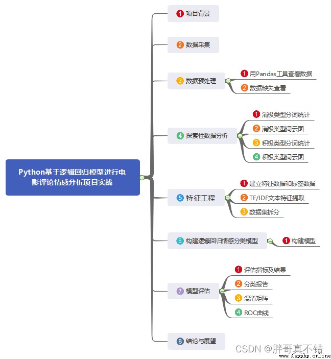
1.項目背景
NLP(自然語言處理)是計算機科學領域以及人工智能領域的一個重要的研究方向,它研究用計算機來處理、理解以及運用人類語言(Such as Chinese and so on),達到人與計算機之間進行有效通訊.所謂“自然”乃是寓意自然進化形成,是為了區分一些人造語言,類似Python、Java等人為設計的語言.在人類社會中,Language plays an important role,Language is the fundamental sign that distinguishes humans from other animals,沒有語言,The human mind is out of the question,Communication is the water without a source.這些年,NLP研究取得了長足的進步,逐漸發展成為一門獨立的學科,從自然語言的角度出發,NLP基本可以分為兩個部分:自然語言處理以及自然語言生成.
This project applies a logistic regression model for sentiment analysis of movie reviews.
2.數據采集
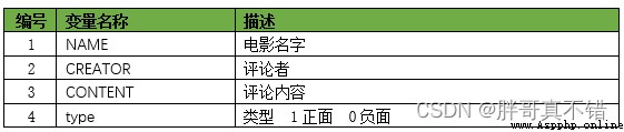
本次建模數據來源於網絡,數據項統計如下:
數據詳情如下(部分展示):
3.數據預處理
3.1用Pandas工具查看數據
使用Pandas工具的head()方法查看前五行數據:
結果如圖所示:
3.2Missing data statistics
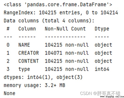
使用Pandas工具的info()The method counts the missing values for each feature:
結果如圖所示:
4.探索性數據分析
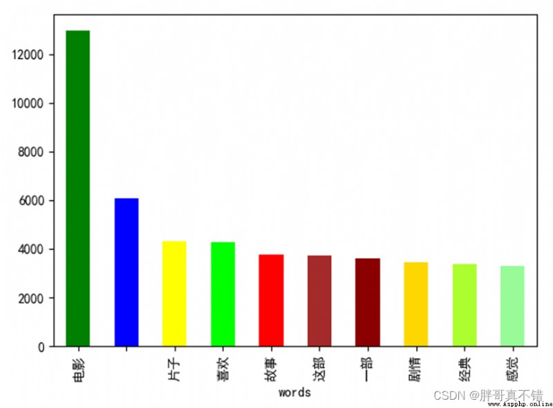
4.1Negative type word segmentation statistics
all_words0 = [i.strip() for line in data_0.CONTENT for i in line.split(',')] # 獲取所有分詞
all_df0 = pd.DataFrame({'words': all_words0}) # 構建數據框
all_df0.groupby(['words'])['words'].count().sort_values(ascending=False)[:10].plot.bar(
color=['green', 'blue', 'yellow', 'lime', 'red', 'brown', 'darkred', 'gold', 'greenyellow',
'palegreen']) # 對分詞進行統計、按降序進行排序 Take the former word frequency before10的分詞
plt.show() # 展示圖片
結果如圖所示:
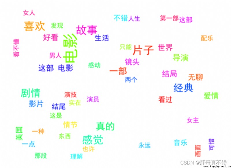
4.2Negative Type word cloud illustration
my_wordcloud0 = wc.generate(list_new0) # 生成詞雲
plt.imshow(my_wordcloud0) # 顯示詞雲
plt.axis("off") # 關閉保存
plt.show()
wc.to_file('Negative word cloud illustration.png')
plt.close() # 關閉當前窗口
結果如圖所示:
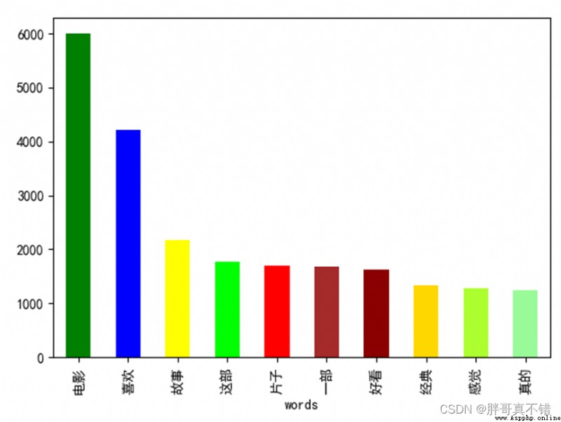
4.3Active type word segmentation statistics
data_1 = data[data['type'] == 1]
all_words1 = [i.strip() for line in data_1.CONTENT for i in line.split(',')] # 獲取所有分詞
all_df1 = pd.DataFrame({'words': all_words1}) # 構建數據框
all_df1.groupby(['words'])['words'].count().sort_values(ascending=False)[:10].plot.bar(
color=['green', 'blue', 'yellow', 'lime', 'red', 'brown', 'darkred', 'gold', 'greenyellow',
'palegreen']) # 對分詞進行統計、按降序進行排序 Take the former word frequency before10的分詞
plt.show() # 展示圖片
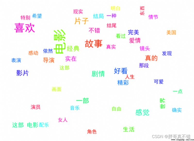
4.4Positive Type word cloud illustration
my_wordcloud1 = wc.generate(list_new1) # 生成詞雲
plt.imshow(my_wordcloud1) # 顯示詞雲
plt.axis("off") # 關閉保存
plt.show()
wc.to_file('Positive word cloud illustration.png') # 保存圖片文件
plt.close() # 關閉當前窗口
結果如圖所示:
5.特征工程
5.1構建特征和標簽
X = data[['CONTENT']] # 構建特征
y = data['type'] # 構建標簽
5.2 TF/IDF文本特征提取
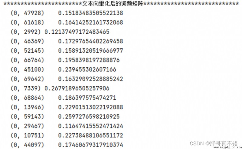
tfidf = TfidfVectorizer() # 文本向量化 除了考量某詞匯在文本出現的頻率,Also focusing on the number of all texts that contain this word can reduce the impact of frequent occurrences of meaningless words, 挖掘更有意義的特征
X_train = tfidf.fit_transform(X_train.CONTENT) # fit transformation
print('***********************Term frequency matrix after text vectorization****************************')
print(X_train[:1, :])
結果如圖所示:
5.3數據集拆分
X_train, X_valid, y_train, y_valid = train_test_split(X, y, test_size=0.2, random_state=42) # 進行數據拆分6.Build a logistic regression sentiment classification model
6.1模型構建
model = LogisticRegression() # 建模
model.fit(X_train, y_train) # 擬合
y_pred = model.predict(X_valid) # 預測
7.模型評估
7.1評估指標及結果
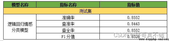
評估指標主要包括准確率、查准率、查全率(召回率)、F1分值等等.
print('Logistic regression classification model-默認參數-Accuracy score: {0:0.4f}'.format(accuracy_score(y_valid, y_pred)))
print("Logistic regression classification model-默認參數-查准率 :", round(precision_score(y_valid, y_pred, average='weighted'), 4), "\n")
print("Logistic regression classification model-默認參數-召回率 :", round(recall_score(y_valid, y_pred, average='weighted'), 4), "\n")
print("Logistic regression classification model-默認參數-F1分值:", round(f1_score(y_valid, y_pred, average='weighted'), 4), "\n")
通過上表可以看到,模型的准確率為85.52%,F1分值為0.8326,說明模型效果良好.
7.2分類報告
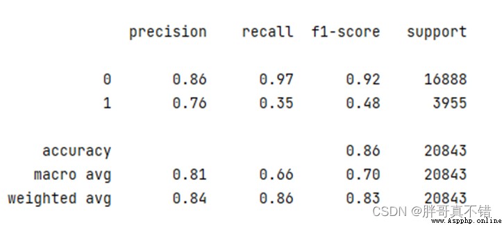
print(classification_report(y_valid, y_pred))
Type is negativeF1分值為0.92;Type is positiveF1分值為0.48.
7.3混淆矩陣
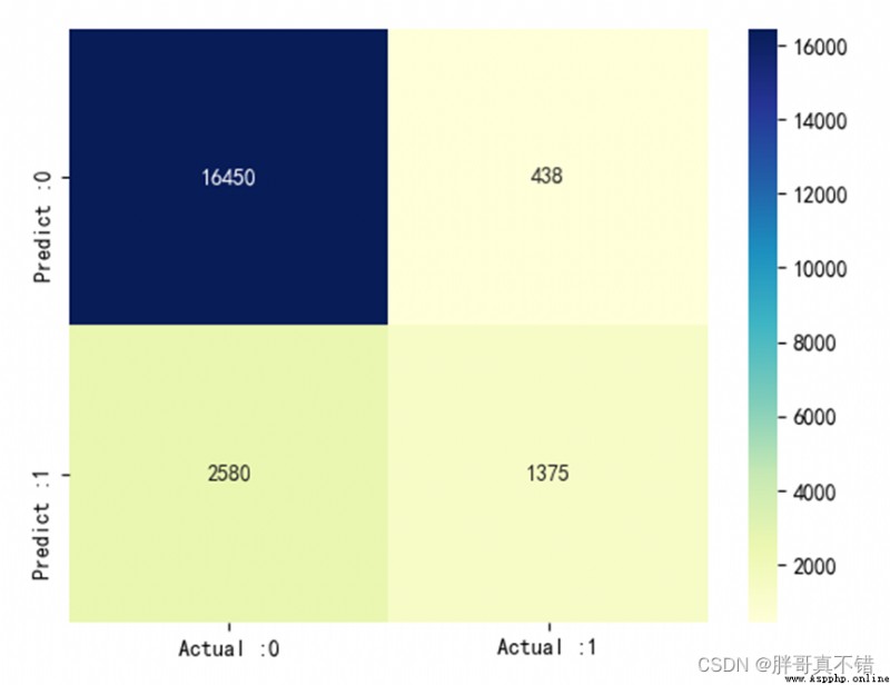
cm_matrix = pd.DataFrame(data=cm, columns=['Actual :0', 'Actual :1'],
index=['Predict :0', 'Predict :1'])
sns.heatmap(cm_matrix, annot=True, fmt='d', cmap='YlGnBu') # 熱力圖展示
plt.show() # 展示圖片
結果如圖所示:
從上圖可以看到,預測為負面 There are actually positive ones428條;預測為正面 actually negative2580條.
7.4ROC曲線
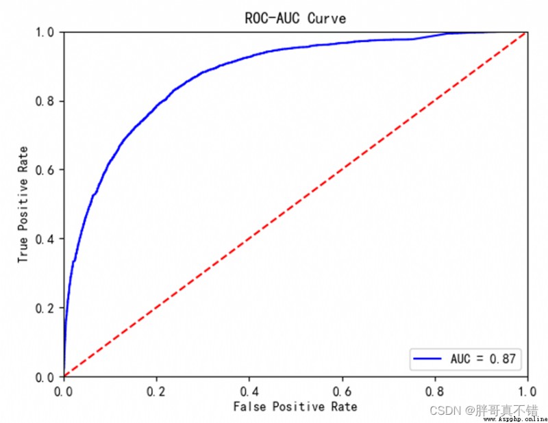
plt.plot(fpr, tpr, 'b', label='AUC = %0.2f' % roc_auc) # 繪制曲線圖
plt.legend(loc='lower right') # 設置圖例
plt.plot([0, 1], [0, 1], 'r--') # 繪制曲線圖
plt.xlim([0, 1]) # 獲取或設置xAxis value display range圍0-1
plt.ylim([0, 1]) # 獲取或設置yAxis value display range0-1
plt.ylabel('True Positive Rate') # 設置y軸名稱
plt.xlabel('False Positive Rate') # 設置x軸名稱
plt.title('ROC-AUC Curve') # 設置標題
plt.show() # 顯示圖片
結果如圖所示:
從上圖可以看到,AUC的值為0.87,說明模型效果良好.
8.總結展望
This project applies logistic regression model to conduct sentiment classification research on movie review data,通過數據預處理、探索性數據分析、特征工程、模型構建、模型評估等工作,最終模型的F1分值達到0.83,這在文本分類領域,is a very good effect,可以應用於實際工作中.
本次機器學習項目實戰所需的資料,項目資源如下:
項目說明:
鏈接:https://pan.baidu.com/s/1dW3S1a6KGdUHK90W-lmA4w
提取碼:bcbp網盤如果失效,可以添加博主微信:zy10178083