文章目錄

• 一 介紹
• • 1 Pandas是什麼
  • 2 Pandas的優勢
• 二 數據結構
• • 1 Series
  • • （1）Series的創建
    • • Build without specifying content,默認索引
      • 指定內容,默認索引
      • 指定內容,指定索引
      • 通過字典數據創建
    • （2）Series的屬性
  • 2 DataFram
  • • （1）DataFrame的創建
    • （2）DataFrame的屬性
    • （3）DatatFrame索引的設置
    • • 修改行列索引值
      • 重設索引
      • 以某列值設置為新的索引
  • 3 MultiIndex
  • • （1）Multiindex特性
    • （2）multiIndex的創建
  • 4 Panel
  • • （1）panel的創建
    • （2）查看panel的數據
• 三 基本數據操作
• • 1 索引操作
  • • （1）直接使用行列索引(先列後行)
    • （2）結合loc或者iloc使用索引
    • （3）使用ix組合索引
  • 2 賦值操作
  • 3 排序
  • • （1）DataFrame排序
    • （2）Series排序
• 四 DataFram運算
• • 1 算數運算
  • 2 邏輯運算
  • • 2.1 邏輯運算符號
    • 2.2 邏輯運算函數
  • 3 統計運算
  • • 3.1 describe
    • 3.2 統計函數
    • 3.3 累計統計函數
  • 4 自定義運算

一 介紹

1 Pandas是什麼

• 2008年WesMcKinney開發出的庫
• 專門用於數據挖掘的開源python庫
• 以Numpy為基礎,借力Numpy模塊在計算方面性能高的優勢
• 基於matplotlib,能夠簡便的畫圖
• 獨特的數據結構

2 Pandas的優勢

• 增強圖表可讀性

• 便捷的數據處理能力

• 讀取文件方便

• 封裝了Matplotlib、Numpy的畫圖和計算

二 數據結構

Pandas中一共有三種數據結構,分別為：Series、DataFrame和MultiIndex（老版本中叫Panel ）.

其中Series是一維數據結構,DataFrame是二維的表格型數據結構,MultiIndex是三維的數據結構.

1 Series

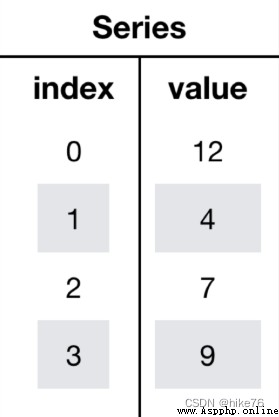
Series是一個類似於一維數組的數據結構,它能夠保存任何類型的數據,比如整數、字符串、浮點數等,主要由一組數據和與之相關的索引兩部分構成.

（1）Series的創建

Build without specifying content,默認索引

# 導入pandas
import pandas as pd
pd.Series(data=None, index=None, dtype=None)

參數說明：

​ data：傳入的數據,可以是ndarray、list等

​ index：索引,必須是唯一的,且與數據的長度相等.如果沒有傳入索引參數,則默認會自動創建一個從0-N的整數索引.

​ dtype：數據的類型

指定內容,默認索引

pd.Series(np.arange(10))
# 運行結果
0 0
1 1
2 2
3 3
4 4
5 5
6 6
7 7
8 8
9 9
dtype: int64

指定內容,指定索引

pd.Series([6.7,5.6,3,10,2], index=[1,2,3,4,5])
# 運行結果
1 6.7
2 5.6
3 3.0
4 10.0
5 2.0
dtype: float64

通過字典數據創建

color_count = pd.Series({
'red':100, 'blue':200, 'green': 500, 'yellow':1000})
color_count
# 運行結果
blue 200
green 500
red 100
yellow 1000
dtype: int64

（2）Series的屬性

為了更方便地操作Series對象中的索引和數據,Series中提供了兩個屬性index和values

index

color_count.index
# 結果
Index(['blue', 'green', 'red', 'yellow'], dtype='object')

values

color_count.values
# 結果
array([ 200, 500, 100, 1000])

也可以使用索引來獲取數據：

color_count[2]
# 結果
100

2 DataFram

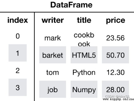
DataFrame是一個類似於二維數組或表格(如excel)的對象,既有行索引,又有列索引

• 行索引,表明不同行,橫向索引,叫index,0軸,axis=0
• 列索引,表名不同列,縱向索引,叫columns,1軸,axis=1
  

（1）DataFrame的創建

# 導入pandas
import pandas as pd
pd.DataFrame(data=None, index=None, columns=None)

參數說明：

​ index：行標簽.如果沒有傳入索引參數,則默認會自動創建一個從0-N的整數索引.

​ columns：列標簽.如果沒有傳入索引參數,則默認會自動創建一個從0-N的整數索引.

不指定index和columns

pd.DataFrame(np.random.randn(2,3))

指定index和columns

# 生成10名同學,5門功課的數據
score = np.random.randint(40, 100, (10, 5))
# 結果
array([[92, 55, 78, 50, 50],
[71, 76, 50, 48, 96],
[45, 84, 78, 51, 68],
[81, 91, 56, 54, 76],
[86, 66, 77, 67, 95],
[46, 86, 56, 61, 99],
[46, 95, 44, 46, 56],
[80, 50, 45, 65, 57],
[41, 93, 90, 41, 97],
[65, 83, 57, 57, 40]])
# 使用Pandas中的數據結構
score_df = pd.DataFrame(score)
# 構造行索引序列
subjects = ["語文", "數學", "英語", "政治", "體育"]
# score_df.shape 值為（10,5）
# score_df.shape[0]值為 10
# score_df.shape[1]值為 5
# Constructs a column index sequence
stu = ['同學' + str(i) for i in range(score_df.shape[0])]
# 添加行列索引
data = pd.DataFrame(score, columns=subjects, index=stu)

（2）DataFrame的屬性

shape：DataFram的維數

data.shape
# 結果
(10, 5)

index：DataFrame的行索引列表

data.index
# 結果
Index(['同學0', '同學1', '同學2', '同學3', '同學4', '同學5', '同學6', '同學7', '同學8', '同學9'], dtype='object')

columns：DataFrame的列索引列表

data.columns
# 結果
Index(['語文', '數學', '英語', '政治', '體育'], dtype='object')

values：直接獲取其中array的值

data.values
array([[92, 55, 78, 50, 50],
[71, 76, 50, 48, 96],
[45, 84, 78, 51, 68],
[81, 91, 56, 54, 76],
[86, 66, 77, 67, 95],
[46, 86, 56, 61, 99],
[46, 95, 44, 46, 56],
[80, 50, 45, 65, 57],
[41, 93, 90, 41, 97],
[65, 83, 57, 57, 40]])

T：Transpose along with row and column labels

data.T

head(5)：顯示前5行內容

如果不補充參數,默認5行.填入參數N則顯示前N行

data.head(5)

tail(5):顯示後5行內容

如果不補充參數,默認5行.填入參數N則顯示後N行

data.tail(5)

（3）DatatFrame索引的設置

修改行列索引值

stu = ["學生_" + str(i) for i in range(score_df.shape[0])]
# 必須整體全部修改
data.index = stu

以下修改方式是錯誤的

# 錯誤修改方式
data.index[3] = '學生_3'

重設索引

reset_index(drop=False)

​ 設置新的下標索引

​ drop:默認為False,不刪除原來索引,如果為True,刪除原來的索引值

# 重置索引,drop=False
data.reset_index()
# 重置索引,drop=True
data.reset_index(drop=True)

以某列值設置為新的索引

set_index(keys, drop=True)

​ keys : 列索引名成或者列索引名稱的列表

​ drop : boolean, default True.當做新的索引,刪除原來的列

# 創建
df = pd.DataFrame({
'month': [1, 4, 7, 10],
'year': [2012, 2014, 2013, 2014],
'sale':[55, 40, 84, 31]})
month sale year
0 1 55 2012
1 4 40 2014
2 7 84 2013
3 10 31 2014
# 以月份設置新的索引
df.set_index('month')
sale year
month
1 55 2012
4 40 2014
7 84 2013
10 31 2014
# 設置多個索引,以年和月份
df = df.set_index(['year', 'month'])
df
sale
year month
2012 1 55
2014 4 40
2013 7 84
2014 10 31

通過剛才的設置,DataFrame就變成了一個具有MultiIndex的DataFrame.

3 MultiIndex

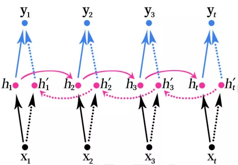
MultiIndex是三維的數據結構

多級索引（也稱層次化索引）是pandas的重要功能,可以在Series、DataFrame對象上擁有2個以及2個以上的索引.

（1）Multiindex特性

# 打印剛才的df的行索引結果
df.index
MultiIndex(levels=[[2012, 2013, 2014], [1, 4, 7, 10]],
labels=[[0, 2, 1, 2], [0, 1, 2, 3]],
names=['year', 'month'])

多級或分層索引對象.

index屬性

​ names:levels的名稱

​ levels：每個level的元組值

df.index.names
# FrozenList(['year', 'month'])
df.index.levels
# FrozenList([[1, 2], [1, 4, 7, 10]])

（2）multiIndex的創建

arrays = [[1, 1, 2, 2], ['red', 'blue', 'red', 'blue']]
pd.MultiIndex.from_arrays(arrays, names=('number', 'color'))
# 結果
MultiIndex(levels=[[1, 2], ['blue', 'red']],
codes=[[0, 0, 1, 1], [1, 0, 1, 0]],
names=['number', 'color'])

4 Panel

（1）panel的創建

class pandas.Panel(data=None, items=None, major_axis=None, minor_axis=None)

​ 作用：存儲3維數組的Panel結構

參數：

data: ndarray或者dataframe

items : 索引或類似數組的對象,axis=0

major_axis: 索引或類似數組的對象,axis=1

minor_axis: 索引或類似數組的對象,axis=2

p = pd.Panel(data=np.arange(24).reshape(4,3,2),
items=list('ABCD'),
major_axis=pd.date_range('20130101', periods=3),
minor_axis=['first', 'second'])
# 結果
<class 'pandas.core.panel.Panel'>
Dimensions: 4 (items) x 3 (major_axis) x 2 (minor_axis)
Items axis: A to D
Major_axis axis: 2013-01-01 00:00:00 to 2013-01-03 00:00:00
Minor_axis axis: first to second

（2）查看panel的數據

p[:,:,"first"]
p["B",:,:]

Pandas從版本0.20.0開始棄用：推薦的用於表示3D數據的方法是通過DataFrame上的MultiIndex方法

三 基本數據操作

使用范例

# 讀取文件
data = pd.read_csv("./data/stock_day.csv")
# 刪除一些列,讓數據更簡單些,再去做後面的操作
data = data.drop(["ma5","ma10","ma20","v_ma5","v_ma10","v_ma20"], axis=1)

1 索引操作

NumpyAmong them, you can use index selection sequence and slice selection,pandas也支持類似的操作,也可以直接使用列名、行名稱,甚至組合使用.

（1）直接使用行列索引(先列後行)

獲取’2018-02-27’這天的’close’的結果

# 直接使用行列索引名字的方式（先列後行）
data['open']['2018-02-27']
23.53
# 不支持的操作
# 錯誤
data['2018-02-27']['open']
# 錯誤
data[:1, :2]

（2）結合loc或者iloc使用索引

獲取從’2018-02-27’:‘2018-02-22’,'open’的結果

# 使用loc:只能指定行列索引的名字
data.loc['2018-02-27':'2018-02-22', 'open']
2018-02-27 23.53
2018-02-26 22.80
2018-02-23 22.88
Name: open, dtype: float64
# 使用iloc可以通過索引的下標去獲取
# 獲取前3天數據,前5列的結果
data.iloc[:3, :5]
open high close low
2018-02-27 23.53 25.88 24.16 23.53
2018-02-26 22.80 23.78 23.53 22.80
2018-02-23 22.88 23.37 22.82 22.71

（3）使用ix組合索引

獲取行第1天到第4天,[‘open’, ‘close’, ‘high’, ‘low’]這個四個指標的結果

# 使用ix進行下表和名稱組合做引
data.ix[0:4, ['open', 'close', 'high', 'low']]
# 推薦使用loc和iloc來獲取的方式
data.loc[data.index[0:4], ['open', 'close', 'high', 'low']]
data.iloc[0:4, data.columns.get_indexer(['open', 'close', 'high', 'low'])]
open close high low
2018-02-27 23.53 24.16 25.88 23.53
2018-02-26 22.80 23.53 23.78 22.80
2018-02-23 22.88 22.82 23.37 22.71
2018-02-22 22.25 22.28 22.76 22.02

Warning:Starting in 0.20.0, the .ix indexer is deprecated, in favor of the more strict .iloc and .loc indexers.

2 賦值操作

對DataFrame當中的closeAll values ​​of the column are reassigned to1

# 直接修改原來的值
data['close'] = 1
# 或者
data.close = 1

3 排序

排序有兩種形式,一種對於索引進行排序,一種對於內容進行排序

（1）DataFrame排序

使用df.sort_values(by=, ascending=)Sort on a single key or on multiple keys,

參數：

​ by：指定排序參考的鍵

​ ascending:默認升序

​ ascending=False:降序

​ ascending=True:升序

# 按照開盤價大小進行排序 , 使用ascending指定按照大小排序
data.sort_values(by="open", ascending=True).head()

Sort by multiple keys,When the first keys are equal,Sort by the second value

# 按照多個鍵進行排序
data.sort_values(by=['open', 'high'])

使用df.sort_index給索引進行排序

這個股票的日期索引原來是從大到小,現在重新排序,從小到大

默認按照升序排序

# 對索引進行排序
data.sort_index().head()

（2）Series排序

使用series.sort_values(ascending=True)進行排序

series排序時,只有一列,不需要參數

data['p_change'].sort_values(ascending=True).head()
2015-09-01 -10.03
2015-09-14 -10.02
2016-01-11 -10.02
2015-07-15 -10.02
2015-08-26 -10.01
Name: p_change, dtype: float64

使用series.sort_index()進行排序,與df一致

# 對索引進行排序
data['p_change'].sort_index().head()
2015-03-02 2.62
2015-03-03 1.44
2015-03-04 1.57
2015-03-05 2.02
2015-03-06 8.51
Name: p_change, dtype: float64

四 DataFram運算

1 算數運算

add(other)

sub(other)

Add all numbers in a column to perform a math operation（減）a specific number

data['open'].add(1)
data['open'] + 1
2018-02-27 24.53
2018-02-26 23.80
2018-02-23 23.88
2018-02-22 23.25
2018-02-14 22.49

2 邏輯運算

2.1 邏輯運算符號

篩選data[“open”] > 23的日期數據：data[“open”] > 23返回邏輯結果

data["open"] > 23
2018-02-27 True
2018-02-26 False
2018-02-23 False
2018-02-22 False
2018-02-14 False
# 邏輯判斷的結果可以作為篩選的依據
data[data["open"] > 23].head()

完成多個邏輯判斷

data[(data["open"] > 23) & (data["open"] < 24)].head()

2.2 邏輯運算函數

query(expr)：expr:查詢字符串

通過query使得剛才的過程更加方便簡單

data.query("open<24 & open>23").head()

isin(values)

例如判斷’open’是否為23.53和23.85

# 可以指定值進行一個判斷,從而進行篩選操作
data[data["open"].isin([23.53, 23.85])]

3 統計運算

3.1 describe

綜合分析: 能夠直接得出很多統計結果,count, mean, std, min, max 等

# 計算平均值、標准差、最大值、最小值
data.describe()

3.2 統計函數

min(最小值), max(最大值), mean(平均值), median(中位數), var(方差), std(標准差),mode(眾數)結果:

countNumber of non-NA observationssumSum of valuesmeanMean of valuesmedianArithmetic median of valuesminMinimummaxMaximummodeModeabsAbsolute ValueprodProduct of valuesstdBessel-corrected sample standard deviationvarUnbiased varianceidxmaxcompute the index labels with the maximumidxmincompute the index labels with the minimum

對於單個函數去進行統計的時候,坐標軸還是按照默認列“columns” (axis=0, default),如果要對行“index” 需要指定(axis=1)

使用對象.The method name can be called

3.3 累計統計函數

函數作用cumsum計算前1/2/3/…/n個數的和cummax計算前1/2/3/…/n個數的最大值cummin計算前1/2/3/…/n個數的最小值cumprod計算前1/2/3/…/n個數的積

These functions can be correctseries和dataframe操作

# 排序之後,進行累計求和
data = data.sort_index()
# 對p_change進行求和
stock_rise = data['p_change']
# plot方法集成了前面直方圖、條形圖、餅圖、折線圖
stock_rise.cumsum()
2015-03-02 2.62
2015-03-03 4.06
2015-03-04 5.63
2015-03-05 7.65
2015-03-06 16.16
2015-03-09 16.37
2015-03-10 18.75
2015-03-11 16.36
2015-03-12 15.03
2015-03-13 17.58
2015-03-16 20.34
2015-03-17 22.42
2015-03-18 23.28
2015-03-19 23.74
2015-03-20 23.48
2015-03-23 23.74
# 使用plot函數,需要導入matplotlib.
import matplotlib.pyplot as plt
# plot顯示圖形
stock_rise.cumsum().plot()
# 需要調用show,才能顯示出結果
plt.show()

4 自定義運算

apply(func, axis=0)

​ func:自定義函數

​ axis=0:默認是列,axis=1為行進行運算

定義一個對列,最大值-最小值的函數

data[['open', 'close']].apply(lambda x: x.max() - x.min(), axis=0)
open 22.74
close 22.85
dtype: float64

匿名函數：lambda x: x.max() - x.min(),將x.max() - x.min()的結果返回給x,使用lambda關鍵字定義