算法簡述:
最小均方算法,簡稱LMS算法,是一種最陡下降算法的改進算法, 是在維納濾波理論上運用速下降法後的優化延伸,最早是由 Widrow 和 Hoff 提出來的。 該算法不需要已知輸入信號和期望信號的統計特征,“當前時刻”的權系數是通過“上一 時刻”權系數再加上一個負均方誤差梯度的比例項求得。 其具有計算復雜程度低、在信號為平穩信號的環境中收斂性好、其期望值無偏地收斂到維納解和利用有限精度實現算法時的平穩性等特性,使LMS算法成為自適應算法中穩定性最好、應用最廣的算法
算法實現步驟:
(1)設置變量和參量:
X(n)為輸入向量,或稱為訓練樣本
W(n)為權值向量
b(n)為偏差
d(n)為期望輸出
y(n)為實際輸出
η為學習速率
n為迭代次數
(2)初始化,賦給w(0)各一個較小的隨機非零值,令n=0
(3)對於一組輸入樣本x(n)和對應的期望輸出d,計算
e(n)=d(n)-X^T(n)W(n)
W(n+1)=W(n)+ηX(n)e(n)
(4)判斷是否滿足條件,若滿足算法結束,若否n增加1,轉入第(3)步繼續執行
實際上我本身是在幫別人做一個題目,題目如下: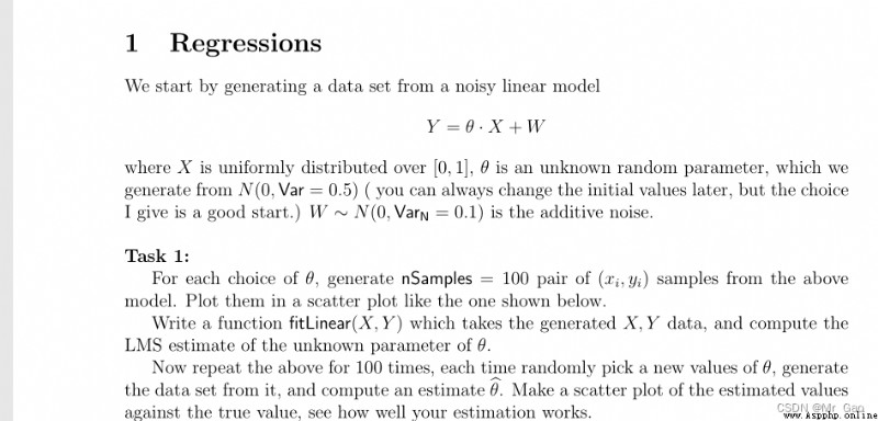
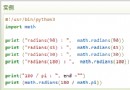
lsm算法實現如下:
def lsm_fit(theta,sample_num,learn_rating):
dim=len(theta)
noise=np.random.normal(0,0.1,(sample_num,dim))
X=np.random.randint(0,100,(sample_num,dim))
Y=X*theta+noise
theta_fit=np.random.normal(0,0.1,(dim))
# print(theta,noise,theta_fit)
loss=[]
for i in range(50):
p=0
for x in X:
e=Y[p]-np.dot(x,theta_fit)
theta_fit=theta_fit+learn_rating*x*e
p=p+1
# print("(theta,theta_fit",theta,theta_fit)
return theta_fit
還是很有趣的一個題目,感興趣的,可以學習一下
上述題目解決如下:
import numpy as np
import os
import matplotlib.pyplot as plt
def lsm_fit(theta,sample_num,learn_rating):
dim=len(theta)
noise=np.random.normal(0,0.1,(sample_num,dim))
X=np.random.randint(0,100,(sample_num,dim))
Y=X*theta+noise
theta_fit=np.random.normal(0,0.1,(dim))
# print(theta,noise,theta_fit)
loss=[]
for i in range(50):
p=0
for x in X:
e=Y[p]-np.dot(x,theta_fit)
theta_fit=theta_fit+learn_rating*x*e
p=p+1
# print("(theta,theta_fit",theta,theta_fit)
return theta_fit
sample_num=100
theta_list=[]
theta_fit_list=[]
x=np.arange(0,100,1)
x.reshape(100,1)
print(x)
for i in range(100):
theta=np.random.normal(0,0.1,(1))
theta_fit=lsm_fit(theta,sample_num,0.00001)
# print("(theta,theta_fit",theta,theta_fit)
theta_list.append(theta)
theta_fit_list.append(theta_fit)
figure, axes = plt.subplots( nrows=1, ncols=2, figsize=(12,8), dpi=80 )
axes[0].plot(x, theta_list, color='r', label = 'theta_list')
axes[1].plot(x, theta_fit_list, color='g', label = 'theta_fit_list')
plt.show()
os.system("pause")
下面是我做的一個實驗結果圖: