PCA Algorithm is a very common algorithm in machine learning and deep learning , I saw this algorithm when I read flower books recently , So after writing the theory, I also want to use some examples to help understand PCA.
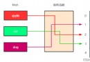
About PCA The theoretical part of the algorithm can Check the boss' article
The following is based on python Self realized PCA Algorithm and use Kaggle Platform Handwritten digital datasets ,
m strip 2 D data pca Get four results : Compressed data 、 The restored data 、 The proportion of each eigenvalue 、 front i The proportion of the sum of eigenvalues def load_data(path=None, m=10000):
if not path:
# m strip 2 D data
x = np.random.randn(m)
y = np.random.randn(m)
data = np.stack([x, y], axis=1) # m, 2
# print(data.shape)
else:
if os.path.basename(path)[-3:] == 'csv':
df = pd.read_csv(path)
data = df.loc[:, df.columns!= 'label']
return np.array(data)
def pca(data, k=99999):
# data: m, n,m strip n D data
mean = np.mean(data, axis=0) # n,
# De centralization
meadnRemoved = data - mean # m, n
# rowvar = 0, Except for m-1
# rowvar = 1, Except for m
cov = np.cov(meadnRemoved, rowvar=0) # n, n
# j Eigenvalues
# n, j j individual n A matrix of dimensional eigenvectors
eigVals, eigVecs = np.linalg.eig(cov)# Decompose and calculate the covariance matrix ( The eigenvalue Eigenvector )
eigValsArgsort = np.argsort(eigVals,)# Default is from small to large
eigValsArgsort = eigValsArgsort[:(-k+1):-1]# Flashback retrieval , Take one of the biggest k individual
decEigVecs = eigVecs[:, eigValsArgsort] # n, k
decData = np.dot(meadnRemoved, decEigVecs) # m, n n, k --> m, k
dataReverse = np.dot(decData, decEigVecs.T) # m, k k, n -->m, n
meanReverse = np.mean(dataReverse, axis=0)
dataReverse = dataReverse + meanReverse # Restore the original data through the reduced dimension data and transformation matrix
eigValsSort = np.sort(eigVals)[::-1] # All eigenvalues are arranged from large to small
eigVals_rotio = eigValsSort / np.sum(eigVals) * 100 # The proportion of each eigenvalue to the sum of all eigenvalues
# front i The ratio of the sum of eigenvalues to the sum of all eigenvalues
eigVals_sum_rotio = np.array([np.sum(eigValsSort[:i]) / np.sum(eigVals) * 100 for i in range(len(eigValsSort))])
return decData, dataReverse, eigVals_rotio, eigVals_sum_rotio
if __name__ == '__main__':
data = load_data(m=1000) # m, 2
decData, dataReverse, ratio, sum_ratio = pca(data, k=1)
# visualization
fig = plt.figure(figsize=(20,10))
ax1 = fig.add_subplot(131)
ax1.scatter(data[:,0],data[:,1],marker='^',s=90) # The original data
ax1.scatter(decData[:,0],np.zeros(len(decData)),c='black',) # Reduced dimension graph
ax1.scatter(dataReverse[:,0],dataReverse[:,1],marker='^',s=50,c='red') # Restored data
plt.legend(['row data','decomposed data','reversed data'])
ax2 = fig.add_subplot(132)
ax2.plot(np.arange(1, len(ratio) + 1),ratio, marker='^')
plt.xticks(np.arange(1, len(ratio) + 1))
plt.legend(['eigvals ratio'])
ax3 = fig.add_subplot(133)
ax3.plot(np.arange(1, len(sum_ratio) + 1), sum_ratio, marker='^')
plt.xticks(np.arange(1, len(sum_ratio) + 1))
plt.legend(['frst i eigvals sum ratio'])
plt.show()
The results are shown in the following figure .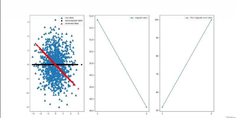
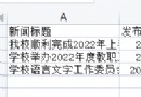
The data set includes three csv file .
sample_submission.csv Is submitted to kaggle Of csv File format .train.csv It's data Training set , Contains 784 Characteristics and 1 Tag columns . common 42000 Group data .test.csv For test set , Contains 784 Features , The dataset No, Label column , common 28000 Group data .
1. Roughly determine the range of the number of principal components .load_data Functions and pca The function does not change , Change the main function to the following code .
if __name__ == '__main__':
path = r'digit-recognizer\train.csv'
data = load_data(path=path) # m, n
decData, dataReverse, ratio, sum_rotio = pca(data,)
fig = plt.figure(figsize=(10,5))
plt.plot(np.arange(1, len(sum_rotio)+1),sum_rotio, )
plt.xticks(np.arange(0, 800, 50))
plt.show()
You can see about 100 The hour has reached 90% Above .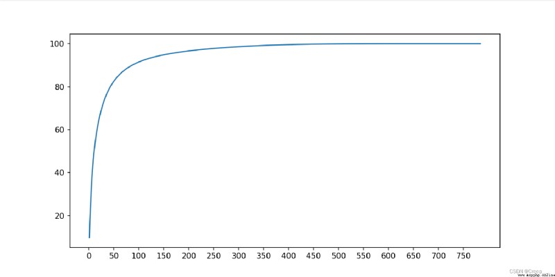
2. Further determine the number of principal components
From the above analysis, we can know that the principal component is 1-100 Between , In order to further determine the number of principal components , Take a different one k Value usage SVM Model to calculate the accuracy of the model , Determine according to the line chart .
ps:SVM Training is really slow ! You can try to change other algorithms .
if __name__ == '__main__':
path = r'digit-recognizer\train.csv'
data, label = load_data(path=path) # m, n
n_components = range(1, 101, 10)
scores = []
for i in tqdm(n_components):
decData, dataReverse, ratio, sum_rotio = pca(data, k=i)
clf = SVC(C=200, kernel='rbf')
clf.fit(decData, label)
print("done!")
# X_new = PCA(n_components=i).fit_transform(X)
scores.append(cross_val_score(clf, decData, label, cv=5).mean())
fig = plt.figure(figsize=(10, 5))
plt.plot(n_components, scores)
plt.xticks(range(0, 101, 10))
plt.show()
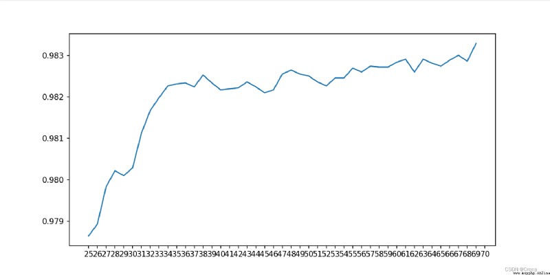
The result is shown in the figure . It can be seen that the approximate number of principal components is (25, 78 The accuracy reaches the saturation value .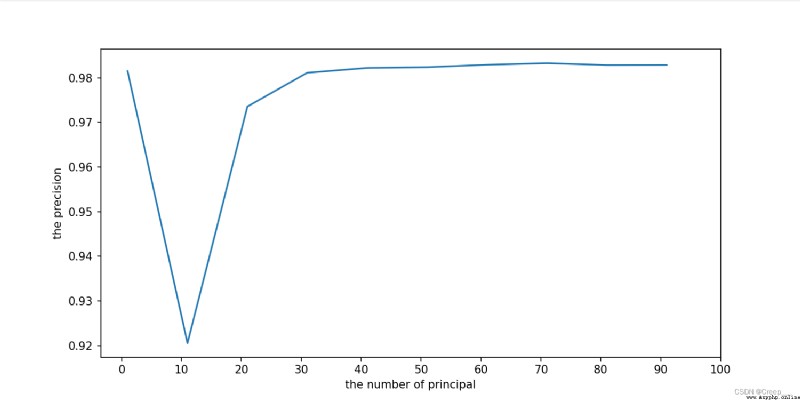
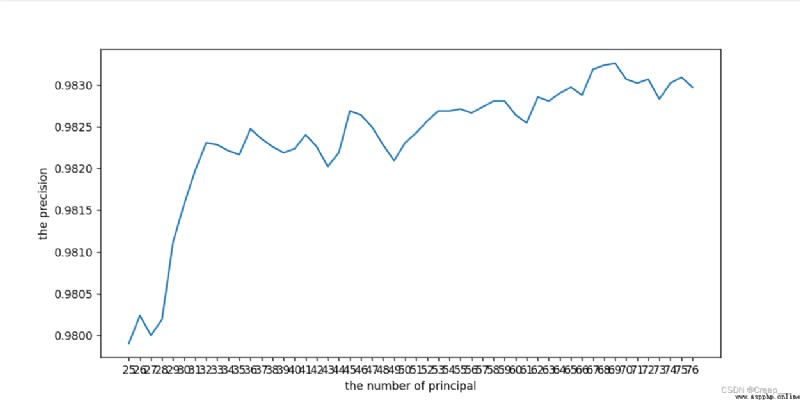
Continue to narrow the scope . For the first time, I only set it to (25, 70, Find out the end 70 At that time, it was still an upward trend , So I ran away again (68,78)
if __name__ == '__main__':
path = r'digit-recognizer\train.csv'
data, label = load_data(path=path) # m, n
n_components = range(25, 78)
scores = []
for i in tqdm(n_components):
decData, dataReverse, ratio, sum_rotio = pca(data, k=i)
clf = SVC(C=200, kernel='rbf')
clf.fit(decData, label)
print("done!")
# X_new = PCA(n_components=i).fit_transform(X)
scores.append(cross_val_score(clf, decData, label, cv=5).mean())
fig = plt.figure(figsize=(10, 5))
plt.plot(n_components, scores)
plt.xticks(range(25, 78))
plt.show()
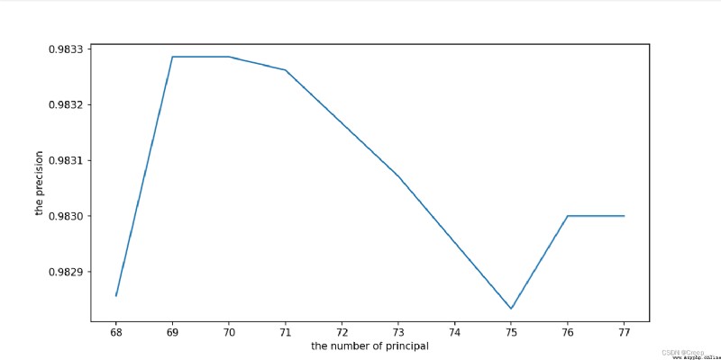
The final choice 70.
if __name__ == '__main__':
path = r'digit-recognizer\train.csv'
data, label = load_data(path=path) # m, n
decData, dataReverse, ratio, sum_rotio = pca(data, k=70)
knn = KNeighborsClassifier()
score = cross_val_score(knn, decData, label, cv=5).mean()
print(score) # 0.9712380952380952
The accuracy can reach 97.12%.
call sklearn Library and its own implementation PCA The calculated results are compared , Found almost the same .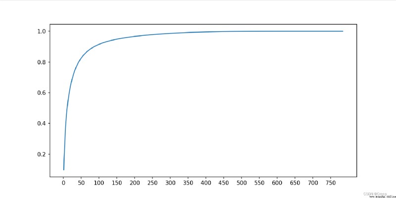
path = r'digit-recognizer\train.csv'
data, label = load_data(path=path) # m, n
n_components = range(25, 77, )
scores = []
for i in tqdm(n_components):
pca_instance = PCA(n_components=i)
decData = pca_instance.fit_transform(data)
ratio = pca_instance.explained_variance_ratio_
sum_rotio = np.cumsum(ratio)
clf = SVC(C=200, kernel='rbf')
clf.fit(decData, label)
print("done!")
# X_new = PCA(n_components=i).fit_transform(X)
scores.append(cross_val_score(clf, decData, label, cv=5).mean())
fig = plt.figure(figsize=(10, 5))
plt.plot(n_components, scores)
plt.xticks(range(25, 77,))
plt.show()