您现在的位置：程式師世界 >> 編程語言 > >> 更多編程語言 >> Python

初學Python 自建6層神經網絡訓練Fashion-MNIST數據集 -- 第一扇門

編輯：Python

一般的深度學習入門例子是MNIST 的訓練和測試，幾乎就算是深度學習領域的 HELLO WORLD 了，但是，有一個問題是，MNIST 太簡單了，初學者閉著眼鏡隨便構造幾層網絡就可以將准確率提升到 90% 以上。但是，初學者這算入門了嗎？

答案是沒有。

現實開發當中的例子可沒有這麼簡單，如果讓初學者直接去上手 VOC 或者是 COCO 這樣的數據集，很可能自己搭建的神經網絡准確率不超過 30%。

是的，如果不用開源的 VGG、GooLeNet、ResNet 等等，也許你手下敲出的代碼命中率還沒有瞎猜高。

這篇文章介紹如何用 Pytorch 訓練一個自建的神經網絡去訓練 Fashion-MNIST 數據集。

Fashion-MNIST

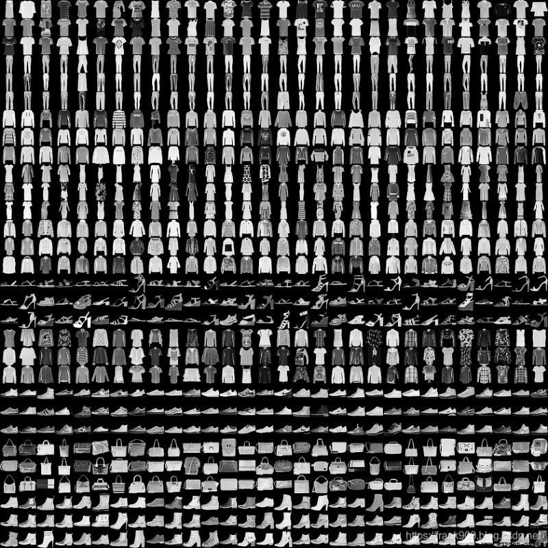
Fashion-MINST 的目的是為了替代 MNIST。

這是它的地址：https://github.com/zalandoresearch/fashion-mnist

它是一系列的服裝圖片集合，總共有 10 個類別。

60000 張訓練圖片，10000 張測試圖片。

LabelDescription0T-shirt/top1Trouser2Pullover3Dress4Coat5Sandal6Shirt7Sneaker8Bag9Ankle boo

Fashion-MNIST 體積並不大，更方便的是像 Tensorflow 和 Pytorch 目前的版本都可以直接用代碼下載。

訓練神經網絡的步驟

下面我張圖是我自己制作的，每次要寫相關博客時，我都會翻出來溫習一下。

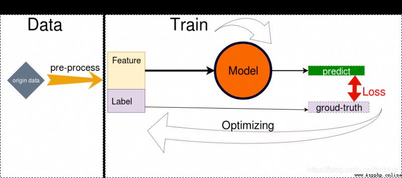
它會提醒我要做這些事情：

處理數據
搭建模型
確定 Loss 函數
訓練

下面文章就按這樣的步驟來講解

處理數據

下載數據

Pytorch 現在通過現成的 API 就可以下載 Fashion-MINST 的數據

trainset = torchvision.datasets.FashionMNIST(root='./data', train=True, download=True, transform=transform)
trainloader = torch.utils.data.DataLoader(trainset, batch_size=100, shuffle=True, num_workers=2)
testset = torchvision.datasets.FashionMNIST(root='./data', train=False, download=True, transform=transform1)
testloader = torch.utils.data.DataLoader(testset, batch_size=50, shuffle=False, num_workers=2)

上面創建了兩個 DataLoader ，分別用來加載訓練集的圖片和測試集的圖片。

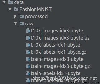
代碼運行後，會在當前目錄的 data 目錄下存放對應的文件。

數據增強

為提高模型的泛化能力，一般會將數據進行增強操作。

transform = transforms.Compose(
[
transforms.RandomHorizontalFlip(),
transforms.RandomGrayscale(),
transforms.ToTensor()])
transform1 = transforms.Compose(
[
transforms.ToTensor()])

transform 主要進行了左右翻轉，灰度隨機變換，用來給訓練的圖像進行數據加強，測試的圖片就不需要了。

transform 的引用傳遞到前面的數據集對應的 API 就可以了，非常方便。

搭建模型

雖然是自己搭建的神經網絡，但是卻參考了 VGG 的網絡架構。

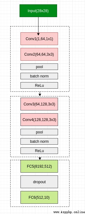
總共 6 層網絡，4 層卷積層，2 層全連接。

用 Pytorch 實現起來也非常方便。

class Net(nn.Module):
def __init__(self):
super(Net,self).__init__()
self.conv1 = nn.Conv2d(1,64,1,padding=1)
self.conv2 = nn.Conv2d(64,64,3,padding=1)
self.pool1 = nn.MaxPool2d(2, 2)
self.bn1 = nn.BatchNorm2d(64)
self.relu1 = nn.ReLU()
self.conv3 = nn.Conv2d(64,128,3,padding=1)
self.conv4 = nn.Conv2d(128, 128, 3,padding=1)
self.pool2 = nn.MaxPool2d(2, 2, padding=1)
self.bn2 = nn.BatchNorm2d(128)
self.relu2 = nn.ReLU()
self.fc5 = nn.Linear(128*8*8,512)
self.drop1 = nn.Dropout2d()
self.fc6 = nn.Linear(512,10)
def forward(self,x):
x = self.conv1(x) # 卷積
x = self.conv2(x)
x = self.pool1(x) # 網絡1
x = self.bn1(x) # 網絡2
x = self.relu1(x) # 網絡3
x = self.conv3(x)
x = self.conv4(x)
x = self.pool2(x) # 網絡4
x = self.bn2(x) # 網絡5
x = self.relu2(x) # 網絡6
#print(" x shape ",x.size())
x = x.view(-1,128*8*8)
x = F.relu(self.fc5(x)) # 全連接1
x = self.drop1(x)
x = self.fc6(x) # 全連接2
return x

值得注意的是，在卷積層後我使用了 Batch Norm 的手段，在全連接層我使用了 Dropout，兩者的目的都是為了降低過擬合的現象。

制定訓練策略

我選用了比較流行的 Adam 作為優化段，學習率 是 0.0001。

然後，loss 選用 交叉熵。

 def train_sgd(self,device,epochs=100):
optimizer = optim.Adam(self.parameters(), lr=0.0001)
path = 'weights.tar'
initepoch = 0
if os.path.exists(path) is not True:
loss = nn.CrossEntropyLoss()
# optimizer = optim.SGD(self.parameters(),lr=0.01)
else:
checkpoint = torch.load(path)
self.load_state_dict(checkpoint['model_state_dict'])
optimizer.load_state_dict(checkpoint['optimizer_state_dict'])
initepoch = checkpoint['epoch']
loss = checkpoint['loss']
for epoch in range(initepoch,epochs): # loop over the dataset multiple times
timestart = time.time()
running_loss = 0.0
total = 0
correct = 0
for i, data in enumerate(trainloader, 0):
# get the inputs
inputs, labels = data
inputs, labels = inputs.to(device),labels.to(device)
# zero the parameter gradients
optimizer.zero_grad()
# forward + backward + optimize
outputs = self(inputs)
l = loss(outputs, labels)
l.backward()
optimizer.step()
# print statistics
running_loss += l.item()
# print("i ",i)
if i % 500 == 499: # print every 500 mini-batches
print('[%d, %5d] loss: %.4f' %
(epoch, i, running_loss / 500))
running_loss = 0.0
_, predicted = torch.max(outputs.data, 1)
total += labels.size(0)
correct += (predicted == labels).sum().item()
print('Accuracy of the network on the %d tran images: %.3f %%' % (total,
100.0 * correct / total))
total = 0
correct = 0
torch.save({
'epoch':epoch,
'model_state_dict':net.state_dict(),
'optimizer_state_dict':optimizer.state_dict(),
'loss':loss
},path)
print('epoch %d cost %3f sec' %(epoch,time.time()-timestart))
print('Finished Training')

上面這段代碼中也有保存和加載模型的功能。

通過 save()
可以保存網絡訓練狀態。

torch.save({
'epoch':epoch,
'model_state_dict':net.state_dict(),
'optimizer_state_dict':optimizer.state_dict(),
'loss':loss
},path)

我在代碼中定義了 path 為 weights.tar，任務執行時，模型數據也會保存下來。
通過load()
可以加載保存的模型數據。

checkpoint = torch.load(path)
self.load_state_dict(checkpoint['model_state_dict'])
optimizer.load_state_dict(checkpoint['optimizer_state_dict'])
initepoch = checkpoint['epoch']
loss = checkpoint['loss']

測試

測試和訓練有些不同，它只需要前向推導就好了。

 def test(self,device):
correct = 0
total = 0
with torch.no_grad():
for data in testloader:
images, labels = data
images, labels = images.to(device), labels.to(device)
outputs = self(images)
_, predicted = torch.max(outputs.data, 1)
total += labels.size(0)
correct += (predicted == labels).sum().item()
print('Accuracy of the network on the 10000 test images: %.3f %%' % (
100.0 * correct / total))

訓練結果

下面編寫代碼進行訓練和驗證。

if __name__ == "__main__":
device = torch.device("cuda:0" if torch.cuda.is_available() else "cpu")
net = Net()
net = net.to(device)
net.train_sgd(device,30)
net.test(device)

代碼會根據機器有沒有 cuda 設備來決定用什麼訓練，比如機器沒有安裝 GPU，那麼就會用 CPU 執行，速度會稍慢一點。

因為模型簡單，我選擇了訓練 30 個 epoch 就終止。

最後，就可以運行代碼了。

我的 Pytorch 版本是 1.2,Cuda 版本是 10.1，GPU 是 1080 Ti.

跑一個 epoch 的時間大概花費 6 秒多。

經過 30 個 epoch 之後，訓練准確度可以達到 99%，測試准確率可以為 92.29%.

[0, 499] loss: 0.4572
Accuracy of the network on the 100 tran images: 87.000 %
epoch 0 cost 7.158301 sec
[1, 499] loss: 0.2840
Accuracy of the network on the 100 tran images: 90.000 %
epoch 1 cost 6.451613 sec
[2, 499] loss: 0.2458
Accuracy of the network on the 100 tran images: 95.000 %
epoch 2 cost 6.450977 sec
[3, 499] loss: 0.2197
Accuracy of the network on the 100 tran images: 92.000 %
epoch 3 cost 6.383819 sec
[4, 499] loss: 0.2009
Accuracy of the network on the 100 tran images: 90.000 %
epoch 4 cost 6.443048 sec
[5, 499] loss: 0.1840
Accuracy of the network on the 100 tran images: 94.000 %
epoch 5 cost 6.411542 sec
[6, 499] loss: 0.1688
Accuracy of the network on the 100 tran images: 94.000 %
epoch 6 cost 6.420368 sec
[7, 499] loss: 0.1584
Accuracy of the network on the 100 tran images: 93.000 %
epoch 7 cost 6.390420 sec
[8, 499] loss: 0.1452
Accuracy of the network on the 100 tran images: 93.000 %
epoch 8 cost 6.473319 sec
[9, 499] loss: 0.1342
Accuracy of the network on the 100 tran images: 96.000 %
epoch 9 cost 6.435586 sec
[10, 499] loss: 0.1275
Accuracy of the network on the 100 tran images: 95.000 %
epoch 10 cost 6.422722 sec
[11, 499] loss: 0.1177
Accuracy of the network on the 100 tran images: 96.000 %
epoch 11 cost 6.490834 sec
[12, 499] loss: 0.1085
Accuracy of the network on the 100 tran images: 96.000 %
epoch 12 cost 6.499629 sec
[13, 499] loss: 0.1021
Accuracy of the network on the 100 tran images: 92.000 %
epoch 13 cost 6.512994 sec
[14, 499] loss: 0.0929
Accuracy of the network on the 100 tran images: 96.000 %
epoch 14 cost 6.510045 sec
[15, 499] loss: 0.0871
Accuracy of the network on the 100 tran images: 94.000 %
epoch 15 cost 6.422577 sec
[16, 499] loss: 0.0824
Accuracy of the network on the 100 tran images: 98.000 %
epoch 16 cost 6.577342 sec
[17, 499] loss: 0.0749
Accuracy of the network on the 100 tran images: 97.000 %
epoch 17 cost 6.491562 sec
[18, 499] loss: 0.0702
Accuracy of the network on the 100 tran images: 99.000 %
epoch 18 cost 6.430238 sec
[19, 499] loss: 0.0634
Accuracy of the network on the 100 tran images: 98.000 %
epoch 19 cost 6.540339 sec
[20, 499] loss: 0.0631
Accuracy of the network on the 100 tran images: 97.000 %
epoch 20 cost 6.490717 sec
[21, 499] loss: 0.0545
Accuracy of the network on the 100 tran images: 98.000 %
epoch 21 cost 6.583902 sec
[22, 499] loss: 0.0535
Accuracy of the network on the 100 tran images: 98.000 %
epoch 22 cost 6.423389 sec
[23, 499] loss: 0.0491
Accuracy of the network on the 100 tran images: 99.000 %
epoch 23 cost 6.573753 sec
[24, 499] loss: 0.0474
Accuracy of the network on the 100 tran images: 95.000 %
epoch 24 cost 6.577250 sec
[25, 499] loss: 0.0422
Accuracy of the network on the 100 tran images: 98.000 %
epoch 25 cost 6.587380 sec
[26, 499] loss: 0.0416
Accuracy of the network on the 100 tran images: 98.000 %
epoch 26 cost 6.595343 sec
[27, 499] loss: 0.0402
Accuracy of the network on the 100 tran images: 99.000 %
epoch 27 cost 6.748190 sec
[28, 499] loss: 0.0366
Accuracy of the network on the 100 tran images: 99.000 %
epoch 28 cost 6.554550 sec
[29, 499] loss: 0.0327
Accuracy of the network on the 100 tran images: 97.000 %
epoch 29 cost 6.475854 sec
Finished Training
Accuracy of the network on the 10000 test images: 92.290 %

92% 是什麼水平呢？在之前給出的 Fashion-MNIST 給出的地址中是可以在 benchmark 排上名的。

網站顯示 Fashion-MNIST 測試的最高分數是 96.7%,說明我這個模型是可以優化和努力的。

後續優化

因為模型是我隨便搭建的，只是吸收了比較先進的手段而已，後續可以在這個基礎上嘗試更多的層數，更少的參數。
耐心的調參，學習率是我隨便給的，是否合理沒有驗證。
ResNet 做圖像識別時，威力比較大，可以嘗試在神經網絡中引入殘差單元。
可視化，也許很多新手會比較沒譜，自己訓練的東西是什麼，那麼你可以自己嘗試把一些中間結果顯示出來。
完整代碼：

import torch
import torch.nn as nn
import torch.nn.functional as F
import torchvision
import torchvision.transforms as transforms
import torch.optim as optim
import time
import os
transform = transforms.Compose(
[
transforms.RandomHorizontalFlip(),
transforms.RandomGrayscale(),
transforms.ToTensor()])
transform1 = transforms.Compose(
[
transforms.ToTensor()])
trainset = torchvision.datasets.FashionMNIST(root='./data', train=True,
download=True, transform=transform)
trainloader = torch.utils.data.DataLoader(trainset, batch_size=100,
shuffle=True, num_workers=2)
testset = torchvision.datasets.FashionMNIST(root='./data', train=False,
download=True, transform=transform1)
testloader = torch.utils.data.DataLoader(testset, batch_size=50,
shuffle=False, num_workers=2)
classes = ('T-shirt', 'Trouser', 'Pullover', 'Dress',
'Coat', 'Sandal', 'Shirt', 'Sneaker', 'Bag', 'Ankle boot')
class Net(nn.Module):
def __init__(self):
super(Net,self).__init__()
self.conv1 = nn.Conv2d(1,64,1,padding=1)
self.conv2 = nn.Conv2d(64,64,3,padding=1)
self.pool1 = nn.MaxPool2d(2, 2)
self.bn1 = nn.BatchNorm2d(64)
self.relu1 = nn.ReLU()
self.conv3 = nn.Conv2d(64,128,3,padding=1)
self.conv4 = nn.Conv2d(128, 128, 3,padding=1)
self.pool2 = nn.MaxPool2d(2, 2, padding=1)
self.bn2 = nn.BatchNorm2d(128)
self.relu2 = nn.ReLU()
self.fc5 = nn.Linear(128*8*8,512)
self.drop1 = nn.Dropout2d()
self.fc6 = nn.Linear(512,10)
def forward(self,x):
x = self.conv1(x)
x = self.conv2(x)
x = self.pool1(x)
x = self.bn1(x)
x = self.relu1(x)
x = self.conv3(x)
x = self.conv4(x)
x = self.pool2(x)
x = self.bn2(x)
x = self.relu2(x)
#print(" x shape ",x.size())
x = x.view(-1,128*8*8)
x = F.relu(self.fc5(x))
x = self.drop1(x)
x = self.fc6(x)
return x
def train_sgd(self,device,epochs=100):
optimizer = optim.Adam(self.parameters(), lr=0.0001)
path = 'weights.tar'
initepoch = 0
if os.path.exists(path) is not True:
loss = nn.CrossEntropyLoss()
# optimizer = optim.SGD(self.parameters(),lr=0.01)
else:
checkpoint = torch.load(path)
self.load_state_dict(checkpoint['model_state_dict'])
optimizer.load_state_dict(checkpoint['optimizer_state_dict'])
initepoch = checkpoint['epoch']
loss = checkpoint['loss']
for epoch in range(initepoch,epochs): # loop over the dataset multiple times
timestart = time.time()
running_loss = 0.0
total = 0
correct = 0
for i, data in enumerate(trainloader, 0):
# get the inputs
inputs, labels = data
inputs, labels = inputs.to(device),labels.to(device)
# zero the parameter gradients
optimizer.zero_grad()
# forward + backward + optimize
outputs = self(inputs)
l = loss(outputs, labels)
l.backward()
optimizer.step()
# print statistics
running_loss += l.item()
# print("i ",i)
if i % 500 == 499: # print every 500 mini-batches
print('[%d, %5d] loss: %.4f' %
(epoch, i, running_loss / 500))
running_loss = 0.0
_, predicted = torch.max(outputs.data, 1)
total += labels.size(0)
correct += (predicted == labels).sum().item()
print('Accuracy of the network on the %d tran images: %.3f %%' % (total,
100.0 * correct / total))
total = 0
correct = 0
torch.save({
'epoch':epoch,
'model_state_dict':net.state_dict(),
'optimizer_state_dict':optimizer.state_dict(),
'loss':loss
},path)
print('epoch %d cost %3f sec' %(epoch,time.time()-timestart))
print('Finished Training')
def test(self,device):
correct = 0
total = 0
with torch.no_grad():
for data in testloader:
images, labels = data
images, labels = images.to(device), labels.to(device)
outputs = self(images)
_, predicted = torch.max(outputs.data, 1)
total += labels.size(0)
correct += (predicted == labels).sum().item()
print('Accuracy of the network on the 10000 test images: %.3f %%' % (
100.0 * correct / total))
if __name__ == "__main__":
device = torch.device("cuda:0" if torch.cuda.is_available() else "cpu")
net = Net()
net = net.to(device)
net.train_sgd(device,30)
net.test(device)