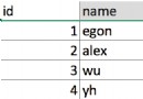
數據源:
一個啤酒的數據源,為了方便演示,數據只有20行。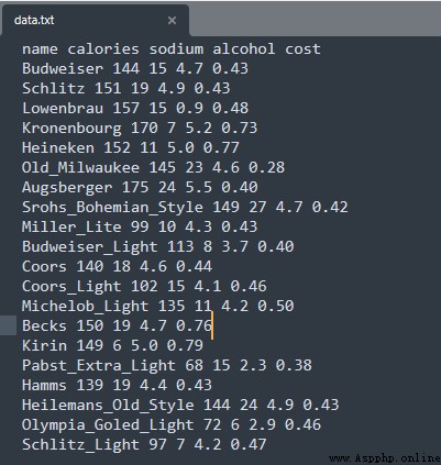
代碼:
import pandas as pd
from sklearn.cluster import KMeans
from pandas.plotting import scatter_matrix
import matplotlib.pyplot as plt
import numpy as np
# 讀取數據源
beer = pd.read_csv('E:/file/data.txt', sep=' ')
X = beer[["calories","sodium","alcohol","cost"]]
# 訓練兩個模型,一個2個簇,一個3個簇
km = KMeans(n_clusters=3).fit(X)
km2 = KMeans(n_clusters=2).fit(X)
# 輸出模型的label
print ("模型的label:" , km.labels_)
# 將標簽新增到數據源上
beer['cluster'] = km.labels_
beer['cluster2'] = km2.labels_
print ("增加聚類標簽後的數據:")
print(beer.sort_values('cluster'))
print ("輸出聚類2各個特征值的均值:")
print(beer.groupby("cluster2").mean())
# pandas 繪制散點圖
cluster_centers = km.cluster_centers_
cluster_centers_2 = km2.cluster_centers_
centers = beer.groupby("cluster").mean().reset_index()
plt.rcParams['font.size'] = 14
colors = np.array(['red', 'green', 'blue', 'yellow'])
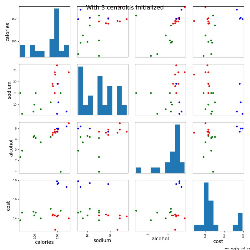
scatter_matrix(beer[["calories","sodium","alcohol","cost"]],s=100, alpha=1, c=colors[beer["cluster"]], figsize=(10,10))
plt.suptitle("With 3 centroids initialized")
plt.show()
測試記錄:
模型的label: [1 1 1 1 1 1 1 1 0 0 1 0 1 1 1 2 1 1 2 0]
增加聚類標簽後的數據:
name calories sodium ... cost cluster cluster2
9 Budweiser_Light 113 8 ... 0.40 0 1
11 Coors_Light 102 15 ... 0.46 0 1
8 Miller_Lite 99 10 ... 0.43 0 1
19 Schlitz_Light 97 7 ... 0.47 0 1
4 Heineken 152 11 ... 0.77 1 0
5 Old_Milwaukee 145 23 ... 0.28 1 0
6 Augsberger 175 24 ... 0.40 1 0
7 Srohs_Bohemian_Style 149 27 ... 0.42 1 0
2 Lowenbrau 157 15 ... 0.48 1 0
10 Coors 140 18 ... 0.44 1 0
1 Schlitz 151 19 ... 0.43 1 0
12 Michelob_Light 135 11 ... 0.50 1 0
13 Becks 150 19 ... 0.76 1 0
14 Kirin 149 6 ... 0.79 1 0
16 Hamms 139 19 ... 0.43 1 0
17 Heilemans_Old_Style 144 24 ... 0.43 1 0
3 Kronenbourg 170 7 ... 0.73 1 0
0 Budweiser 144 15 ... 0.43 1 0
18 Olympia_Goled_Light 72 6 ... 0.46 2 1
15 Pabst_Extra_Light 68 15 ... 0.38 2 1
[20 rows x 7 columns]
輸出聚類2各個特征值的均值:
calories sodium alcohol cost cluster
cluster2
0 150.000000 17.000000 4.521429 0.520714 1.000000
1 91.833333 10.166667 3.583333 0.433333 0.666667

代碼:
import pandas as pd
from sklearn.cluster import KMeans
from pandas.plotting import scatter_matrix
import matplotlib.pyplot as plt
import numpy as np
from sklearn.preprocessing import StandardScaler
# 讀取數據源
beer = pd.read_csv('E:/file/data.txt', sep=' ')
X = beer[["calories","sodium","alcohol","cost"]]
# 對數據進行與處理
scaler = StandardScaler()
X_scaled = scaler.fit_transform(X)
print ("歸一化後的數據集:" )
print(X_scaled)
# 訓練兩個模型,一個2個簇,一個3個簇
km = KMeans(n_clusters=3).fit(X_scaled)
km2 = KMeans(n_clusters=2).fit(X_scaled)
# 輸出模型的label
print ("模型的label:" , km.labels_)
# 將標簽新增到數據源上
beer['cluster'] = km.labels_
beer['cluster2'] = km2.labels_
print ("增加聚類標簽後的數據:")
print(beer.sort_values('cluster'))
print ("輸出聚類2各個特征值的均值:")
print(beer.groupby("cluster2").mean())
# pandas 繪制散點圖
cluster_centers = km.cluster_centers_
cluster_centers_2 = km2.cluster_centers_
centers = beer.groupby("cluster").mean().reset_index()
plt.rcParams['font.size'] = 14
colors = np.array(['red', 'green', 'blue', 'yellow'])
scatter_matrix(beer[["calories","sodium","alcohol","cost"]],s=100, alpha=1, c=colors[beer["cluster"]], figsize=(10,10))
plt.suptitle("With 3 centroids initialized")
plt.show()
測試記錄:
歸一化後的數據集:
[[ 0.38791334 0.00779468 0.43380786 -0.45682969]
[ 0.6250656 0.63136906 0.62241997 -0.45682969]
[ 0.82833896 0.00779468 -3.14982226 -0.10269815]
[ 1.26876459 -1.23935408 0.90533814 1.66795955]
[ 0.65894449 -0.6157797 0.71672602 1.95126478]
[ 0.42179223 1.25494344 0.3395018 -1.5192243 ]
[ 1.43815906 1.41083704 1.1882563 -0.66930861]
[ 0.55730781 1.87851782 0.43380786 -0.52765599]
[-1.1366369 -0.7716733 0.05658363 -0.45682969]
[-0.66233238 -1.08346049 -0.5092527 -0.66930861]
[ 0.25239776 0.47547547 0.3395018 -0.38600338]
[-1.03500022 0.00779468 -0.13202848 -0.24435076]
[ 0.08300329 -0.6157797 -0.03772242 0.03895447]
[ 0.59118671 0.63136906 0.43380786 1.88043848]
[ 0.55730781 -1.39524768 0.71672602 2.0929174 ]
[-2.18688263 0.00779468 -1.82953748 -0.81096123]
[ 0.21851887 0.63136906 0.15088969 -0.45682969]
[ 0.38791334 1.41083704 0.62241997 -0.45682969]
[-2.05136705 -1.39524768 -1.26370115 -0.24435076]
[-1.20439469 -1.23935408 -0.03772242 -0.17352445]]
模型的label: [0 0 1 2 2 0 0 0 1 1 0 1 1 2 2 1 0 0 1 1]
增加聚類標簽後的數據:
name calories sodium ... cost cluster cluster2
0 Budweiser 144 15 ... 0.43 0 1
1 Schlitz 151 19 ... 0.43 0 1
17 Heilemans_Old_Style 144 24 ... 0.43 0 1
16 Hamms 139 19 ... 0.43 0 1
5 Old_Milwaukee 145 23 ... 0.28 0 1
6 Augsberger 175 24 ... 0.40 0 1
7 Srohs_Bohemian_Style 149 27 ... 0.42 0 1
10 Coors 140 18 ... 0.44 0 1
15 Pabst_Extra_Light 68 15 ... 0.38 1 0
12 Michelob_Light 135 11 ... 0.50 1 1
11 Coors_Light 102 15 ... 0.46 1 0
9 Budweiser_Light 113 8 ... 0.40 1 0
8 Miller_Lite 99 10 ... 0.43 1 0
2 Lowenbrau 157 15 ... 0.48 1 0
18 Olympia_Goled_Light 72 6 ... 0.46 1 0
19 Schlitz_Light 97 7 ... 0.47 1 0
13 Becks 150 19 ... 0.76 2 1
14 Kirin 149 6 ... 0.79 2 1
4 Heineken 152 11 ... 0.77 2 1
3 Kronenbourg 170 7 ... 0.73 2 1
[20 rows x 7 columns]
輸出聚類2各個特征值的均值:
calories sodium alcohol cost cluster
cluster2
0 101.142857 10.857143 3.2 0.440000 1.000000
1 149.461538 17.153846 4.8 0.523846 0.692308
計算樣本i到同簇其他樣本的平均距離ai。ai 越小,說明樣本i越應該被聚類到該簇。將ai 稱為樣本i的簇內不相似度。
計算樣本i到其他某簇Cj 的所有樣本的平均距離bij,稱為樣本i與簇Cj 的不相似度。定義為樣本i的簇間不相似度:bi =min{bi1, bi2, …, bik}
si接近1,則說明樣本i聚類合理
si接近-1,則說明樣本i更應該分類到另外的簇
若si 近似為0,則說明樣本i在兩個簇的邊界上。
代碼:
import pandas as pd
from sklearn.cluster import KMeans
from pandas.plotting import scatter_matrix
import matplotlib.pyplot as plt
import numpy as np
from sklearn.preprocessing import StandardScaler
from sklearn import metrics
# 讀取數據源
beer = pd.read_csv('E:/file/data.txt', sep=' ')
X = beer[["calories","sodium","alcohol","cost"]]
# 對數據進行與處理
scaler = StandardScaler()
X_scaled = scaler.fit_transform(X)
# 訓練兩個模型,一個是原始數據,一個是歸一化後的數據
km = KMeans(n_clusters=3).fit(X)
km2 = KMeans(n_clusters=2).fit(X_scaled)
# 將標簽新增到數據源上
beer['cluster'] = km.labels_
beer['scaled_cluster'] = km2.labels_
score_scaled = metrics.silhouette_score(X,beer.scaled_cluster)
score = metrics.silhouette_score(X,beer.cluster)
print("輸出歸一化評分及原始數據樣本評分:")
print(score_scaled, score)
# 查看不同K值下的評分
scores = []
for k in range(2,20):
labels = KMeans(n_clusters=k).fit(X).labels_
score = metrics.silhouette_score(X, labels)
scores.append(score)
print("查看不同K值評分:")
print(scores)
plt.plot(list(range(2,20)), scores)
plt.xlabel("Number of Clusters Initialized")
plt.ylabel("Sihouette Score")
plt.show()
測試記錄:
輸出歸一化評分及原始數據樣本評分:
0.5562170983766765 0.6731775046455796
查看不同K值評分:
[0.6917656034079486, 0.6731775046455796, 0.5857040721127795, 0.422548733517202, 0.4559182167013377, 0.43776116697963124, 0.38946337473125997, 0.39746405172426014, 0.3915697409245163, 0.41282646329875183, 0.3459775237127248, 0.31221439248428434, 0.30707782144770296, 0.31834561839139497, 0.2849514001174898, 0.23498077333071996, 0.1588091017496281, 0.08423051380151177]
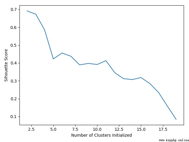
分析:
歸一化之後,居然效果沒有原始數據集好,估計是樣本太簡單了吧,多數情況下作了歸一化之後,效果會有一定程度的提升。