這兩年開始畢業設計和畢業答辯的要求和難度不斷提升,傳統的畢設題目缺少創新和亮點,往往達不到畢業答辯的要求,這兩年不斷有學弟學妹告訴學長自己做的項目系統達不到老師的要求。
為了大家能夠順利以及最少的精力通過畢設,學長分享優質畢業設計項目,今天要分享的是
基於深度學習的數學公式識別算法實現
學長這裡給一個題目綜合評分(每項滿分5分)
🧿 選題指導, 項目分享:
https://gitee.com/dancheng-senior/project-sharing-1/blob/master/%E6%AF%95%E8%AE%BE%E6%8C%87%E5%AF%BC/README.md
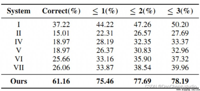
手寫數學公式識別較傳統OCR問題而言,是一個更復雜的二維手寫識別問題,其內部復雜的二維空間結構使得其很難被解析,傳統方法的識別效果不佳。隨著深度學習在各領域的成功應用,基於深度學習的端到端離線數學公式算法,並在公開數據集上較傳統方法獲得了顯著提升,開辟了全新的數學公式識別框架。然而在線手寫數學公式識別框架還未被提出,論文TAP則是首個基於深度學習的端到端在線手寫數學公式識別模型,且針對數學公式識別的任務特性提出了多種優化。
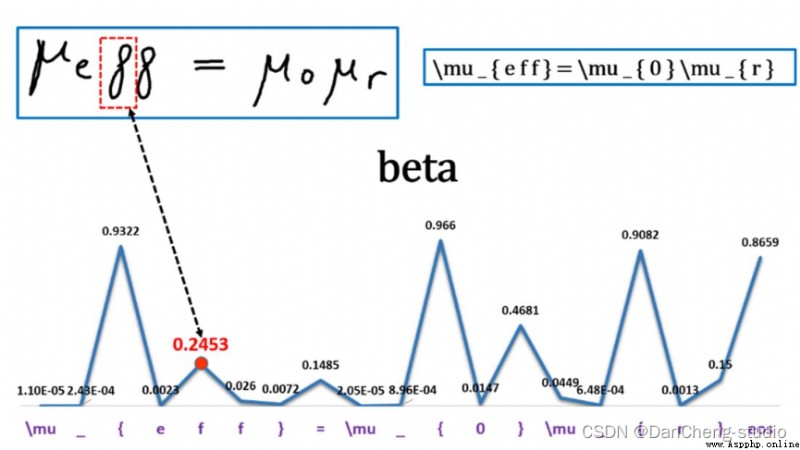
公式識別是OCR領域一個非常有挑戰性的工作,工作的難點在於它是一個二維的數據,因此無法用傳統的CRNN進行識別。
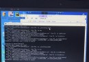
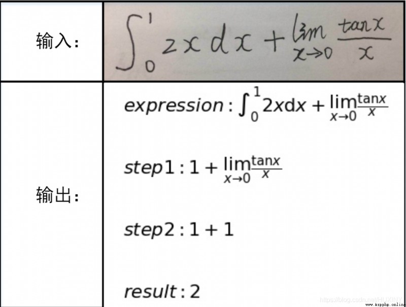
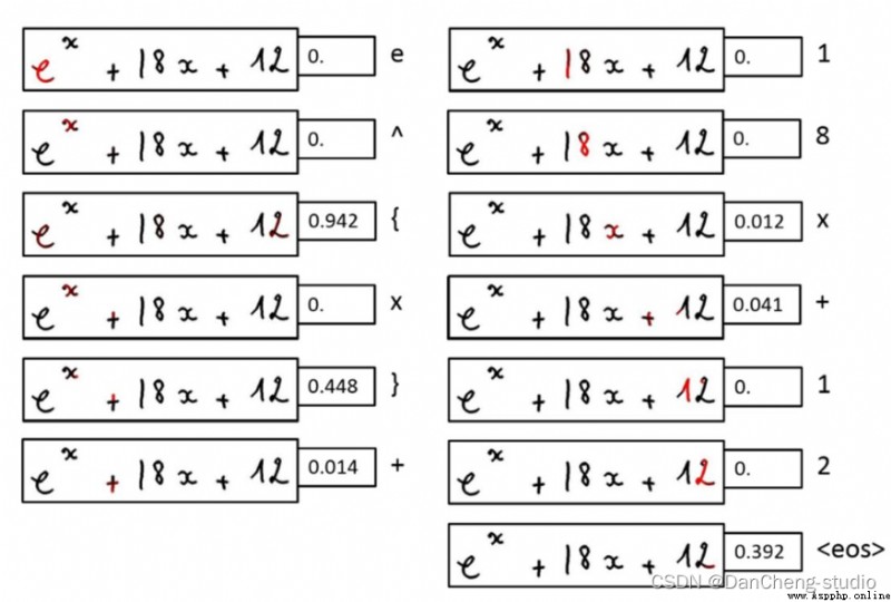
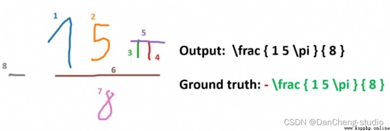
這裡簡單的展示一下效果

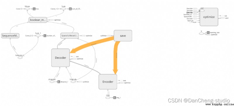
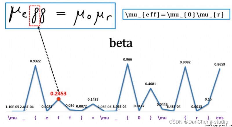
神經網絡模型是 Seq2Seq + Attention + Beam Search。Seq2Seq的Encoder是CNN,Decoder是LSTM。Encoder和Decoder之間插入Attention層,具體操作是這樣:Encoder到Decoder有個扁平化的過程,Attention就是在這裡插入的。具體模型的可視化結果如下
class Encoder(object):
"""Class with a __call__ method that applies convolutions to an image"""
def __init__(self, config):
self._config = config
def __call__(self, img, dropout):
"""Applies convolutions to the image Args: img: batch of img, shape = (?, height, width, channels), of type tf.uint8 tf.uint8 因為 2^8 = 256,所以元素值區間 [0, 255],線性壓縮到 [-1, 1] 上就是 img = (img - 128) / 128 Returns: the encoded images, shape = (?, h', w', c') """
with tf.variable_scope("Encoder"):
img = tf.cast(img, tf.float32) - 128.
img = img / 128.
with tf.variable_scope("convolutional_encoder"):
# conv + max pool -> /2
# 64 個 3*3 filters, strike = (1, 1), output_img.shape = ceil(L/S) = ceil(input/strike) = (H, W)
out = tf.layers.conv2d(img, 64, 3, 1, "SAME", activation=tf.nn.relu)
image_summary("out_1_layer", out)
out = tf.layers.max_pooling2d(out, 2, 2, "SAME")
# conv + max pool -> /2
out = tf.layers.conv2d(out, 128, 3, 1, "SAME", activation=tf.nn.relu)
image_summary("out_2_layer", out)
out = tf.layers.max_pooling2d(out, 2, 2, "SAME")
# regular conv -> id
out = tf.layers.conv2d(out, 256, 3, 1, "SAME", activation=tf.nn.relu)
image_summary("out_3_layer", out)
out = tf.layers.conv2d(out, 256, 3, 1, "SAME", activation=tf.nn.relu)
image_summary("out_4_layer", out)
if self._config.encoder_cnn == "vanilla":
out = tf.layers.max_pooling2d(out, (2, 1), (2, 1), "SAME")
out = tf.layers.conv2d(out, 512, 3, 1, "SAME", activation=tf.nn.relu)
image_summary("out_5_layer", out)
if self._config.encoder_cnn == "vanilla":
out = tf.layers.max_pooling2d(out, (1, 2), (1, 2), "SAME")
if self._config.encoder_cnn == "cnn":
# conv with stride /2 (replaces the 2 max pool)
out = tf.layers.conv2d(out, 512, (2, 4), 2, "SAME")
# conv
out = tf.layers.conv2d(out, 512, 3, 1, "VALID", activation=tf.nn.relu)
image_summary("out_6_layer", out)
if self._config.positional_embeddings:
# from tensor2tensor lib - positional embeddings
# 嵌入位置信息(positional)
# 後面將會有一個 flatten 的過程,會丟失掉位置信息,所以現在必須把位置信息嵌入
# 嵌入的方法有很多,比如加,乘,縮放等等,這裡用 tensor2tensor 的實現
out = add_timing_signal_nd(out)
image_summary("out_7_layer", out)
return out
學長編碼的部分采用的是傳統的卷積神經網絡,該網絡主要有6層組成,最終得到[N x H x W x C ]大小的特征。
其中:N表示數據的batch數;W、H表示輸出的大小,這裡W,H是不固定的,從數據集的輸入來看我們的輸入為固定的buckets,具體如何解決得到不同解碼維度的問題稍後再講;
C為輸入的通道數,這裡最後得到的通道數為512。
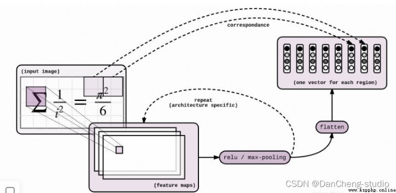
當我們得到特征圖之後,我們需要進行reshape操作對特征圖進行扁平化,代碼具體操作如下:
N = tf.shape(img)[0]
H, W = tf.shape(img)[1], tf.shape(img)[2] # image
C = img.shape[3].value # channels
self._img = tf.reshape(img, shape=[N, H*W, C])
當我們在進行解碼的時候,我們可以直接運用seq2seq來得到我們想要的結果,這個結果可能無法達到我們的預期。因為這個過程會相應的丟失一些位置信息。
位置信息嵌入(Positional Embeddings)
通過位置信息的嵌入,我不需要增加額外的參數的情況下,通過計算512維的向量來表示該圖片的位置信息。具體計算公式如下:

其中:p為位置信息;f為頻率參數。從上式可得,圖像中的像素的相對位置信息可由sin()或cos表示。
我們知道,sin(a+b)或cos(a+b)可由cos(a)、sin(a)、cos(b)以及sin(b)等表示。也就是說sin(a+b)或cos(a+b)與cos(a)、sin(a)、cos(b)以及sin(b)線性相關,這也可以看作用像素的相對位置正、余弦信息來等效計算相對位置的信息的嵌入。
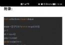
這個計算過程在tensor2tensor庫中已經實現,下面我們看看代碼是怎麼進行位置信息嵌入。代碼實現位於:/model/components/positional.py。
def add_timing_signal_nd(x, min_timescale=1.0, max_timescale=1.0e4):
static_shape = x.get_shape().as_list() # [20, 14, 14, 512]
num_dims = len(static_shape) - 2 # 2
channels = tf.shape(x)[-1] # 512
num_timescales = channels // (num_dims * 2) # 512 // (2*2) = 128
log_timescale_increment = (
math.log(float(max_timescale) / float(min_timescale)) /
(tf.to_float(num_timescales) - 1)) # -0.1 / 127
inv_timescales = min_timescale * tf.exp(
tf.to_float(tf.range(num_timescales)) * -log_timescale_increment) # len == 128 計算128個維度方向的頻率信息
for dim in range(num_dims): # dim == 0; 1
length = tf.shape(x)[dim + 1] # 14 獲取特征圖寬/高
position = tf.to_float(tf.range(length)) # len == 14 計算x或y方向的位置信息[0,1,2...,13]
scaled_time = tf.expand_dims(position, 1) * tf.expand_dims(
inv_timescales, 0) # pos = [14, 1], inv = [1, 128], scaled_time = [14, 128] 計算頻率信息與位置信息的乘積
signal = tf.concat([tf.sin(scaled_time), tf.cos(scaled_time)], axis=1) # [14, 256] 合並兩個方向的位置信息向量
prepad = dim * 2 * num_timescales # 0; 256
postpad = channels - (dim + 1) * 2 * num_timescales # 512-(1;2)*2*128 = 256; 0
signal = tf.pad(signal, [[0, 0], [prepad, postpad]]) # [14, 512] 分別在矩陣的上下左右填充0
for _ in range(1 + dim): # 1; 2
signal = tf.expand_dims(signal, 0)
for _ in range(num_dims - 1 - dim): # 1, 0
signal = tf.expand_dims(signal, -2)
x += signal # [1, 14, 1, 512]; [1, 1, 14, 512]
return x
得到公式圖片x,y方向的位置信息後,只需要要將其添加到原始特征圖像上即可。
🧿 選題指導, 項目分享:
https://gitee.com/dancheng-senior/project-sharing-1/blob/master/%E6%AF%95%E8%AE%BE%E6%8C%87%E5%AF%BC/README.md
🧿 選題指導, 項目分享:
https://gitee.com/dancheng-senior/project-sharing-1/blob/master/%E6%AF%95%E8%AE%BE%E6%8C%87%E5%AF%BC/README.md