I tried it python Process and plot Arctic snow water equivalent data ( source : Arctic snow water equivalent grid dataset ,, In the past, I was used to data processing and image rendering matlab or R, Draw using ArcGIS. however python After all, it's the golden language , Try how to deal with , It's better to prepare for a rainy day in the future , It's like programming reconstruction .
online python There is a lot of code to process and draw , I looked , It feels messy and concise , And lack of polar projection , For the possible problems and the introduction of the whole process, I haven't found any satisfactory information at present , Decided to write a note now for your own use .
nc Data is the most commonly used data type in meteorology , Both reanalysis data and model results are stored in this kind of data , Its processing and visualization process is also the basic operation , I hope this blog can help beginners , After all, drawing and data processing are the most basic content , The code involved is also very simple , Let me summarize briefly here .
This article includes :
1、netcdf4 Library pair nc Simply read, write and process data
2、matplotlib and Cartopy Visualizing data
3、matplotlib Library drawing details
4、 Supplementary content : Use numpy Library for longitude and latitude conversion
You can check in different parts according to your needs .
First, download the right nc Read the data , And look at nc Information , For subsequent processing
import numpy as np
import netCDF4 as nc
d=nc.Dataset('E:/arctic/XDA19070302_154/Arctic_SWE_2019.nc')# Read nc data ,2019 Pan Arctic snow water equivalent data in
all_vars = d.variables.keys() # Get all variable names
all_vars_info = d.variables.items() # Get all variable information
print(type(all_vars_info)) # Output is : odict_items . Here it is translated into list list
all_vars_info = list(all_vars_info)
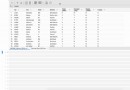
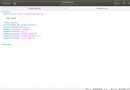
print(all_vars_info) # Show nc Data and information
Got nc The data information is :
<class 'dict_items'>
[('time', <class 'netCDF4._netCDF4.Variable'>
float64 time(time)
standard_name: time
long_name: time
units: days since 2019-01-01
calendar: standard
axis: T
unlimited dimensions: time
current shape = (365,)
filling off), ('x', <class 'netCDF4._netCDF4.Variable'>
float32 x(x)
standard_name: projection_x_coordinate
long_name: x coordinate of projection
units: m
axis: X
unlimited dimensions:
current shape = (978,)
filling off), ('y', <class 'netCDF4._netCDF4.Variable'>
float32 y(y)
standard_name: projection_y_coordinate
long_name: y coordinate of projection
units: m
axis: Y
unlimited dimensions:
current shape = (978,)
filling off), ('lambert_azimuthal_equal_area', <class 'netCDF4._netCDF4.Variable'>
int32 lambert_azimuthal_equal_area()
grid_mapping_name: lambert_azimuthal_equal_area
false_easting: 0.0
false_northing: 0.0
latitude_of_projection_origin: 90.0
longitude_of_projection_origin: 0.0
long_name: CRS definition
longitude_of_prime_meridian: 0.0
semi_major_axis: 6378137.0
inverse_flattening: 298.257223563
spatial_ref: PROJCS["unknown",GEOGCS["unknown",DATUM["WGS_1984",SPHEROID["WGS 84",6378137,298.257223563,AUTHORITY["EPSG","7030"]],AUTHORITY["EPSG","6326"]],PRIMEM["Greenwich",0,AUTHORITY["EPSG","8901"]],UNIT["degree",0.0174532925199433,AUTHORITY["EPSG","9122"]]],PROJECTION["Lambert_Azimuthal_Equal_Area"],PARAMETER["latitude_of_center",90],PARAMETER["longitude_of_center",0],PARAMETER["false_easting",0],PARAMETER["false_northing",0],UNIT["metre",1,AUTHORITY["EPSG","9001"]],AXIS["Easting",SOUTH],AXIS["Northing",SOUTH]]
GeoTransform: -4889336.08287 10000 0 4890662.63721 0 -10000
unlimited dimensions:
current shape = ()
filling off), ('swe', <class 'netCDF4._netCDF4.Variable'>
float64 swe(time, y, x)
grid_mapping: lambert_azimuthal_equal_area
_FillValue: -9999.0
missing_value: -9999.0
unlimited dimensions: time
current shape = (365, 978, 978)
filling off)]
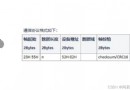
read nc Information , We should pay attention to the following information : Variable 、 Variable dimension 、 Geographic Information .
In this article nc In the data , We have it in common 4 A variable :time( Time , everyday )、x( Projection x coordinate , longitude )y( Projection y coordinate )、swe( Snow water equivalent , It's time 、x and y Commonly described functions ),shape Is the dimension of the variable .
below , We begin to extract variables , And make simple calculations , What we need to do is : according to 2019 Daily snow water equivalent data , Calculation 2019 Annual average snow water equivalent data .
time=np.array(d.variables['time'])# Time
d_lon=np.array(d.variables['x'])# longitude
d_lat=np.array(d.variables['y'])# dimension
swe=np.array(d.variables['swe'])#x Snow water equivalent
FillValue_E=d.variables['swe']._FillValue# There are filling and missing data in snow water equivalent , Find it
print(FillValue_E)
swe=np.ma.masked_values(swe,FillValue_E)# Cover the filled part , Easy to calculate
swe_year=np.transpose(np.sum(swe,axis=0))# take SWE Add according to the time dimension ,axis=0 To sum by columns , Transpose the data after summing , Otherwise, the longitude and latitude will be disordered when drawing
swe_year=np.ma.filled(swe_year,FillValue_E# Refill the annual snow water equivalent , Easy to output
Okay , We calculated 2019 Pan Arctic in (45°N-90°N) Annual snow water equivalent in the region , Next we save it , Easy to use later .
f_w = nc.Dataset('E:/arctic/XDA19070302_154/swe_year.nc','w',format = 'NETCDF4') # Create a format of .nc Of , The name is ‘swe_year.nc’ The file of
f_w.createDimension('x',978) # Set a variable x dimension
f_w.createDimension('y',978) # Set a variable y dimension
f_w.createVariable('x',np.float32,('x')) # Create variables x, For a length of 978, The data type is float32 Array of
f_w.createVariable('y',np.float32,('y'))# ditto
f_w.variables['x'][:] = d_lon# Appoint x value
f_w.variables['y'][:] = d_lat# Appoint y value
f_w.createVariable( 'swe_year', np.float64, ('x','y'))# Create variables swe_year, By variable x And have a description
f_w.variables['swe_year'][:] = swe_year# assignment
f_w.close()
That's all nc Basic operation of data .
cartopy And Matplotlib Relationship
About Cartopy Basic drawing process , There are many materials on the Internet , Here I recommend one :Cartopy Entry to give up
simply ,Cartipy Draw the base map of the map , and Matplotlib Is responsible for drawing the data on the map .
When drawing figures , You need to know : Canvas size 、 Map projection 、 Map display range 、 Data projection method ( important )
If the projection setting is wrong , Or there is a problem with the setting of longitude and latitude range , It will cause your map to have only the bottom map , It will also affect the aesthetics of the drawing ( The lesson of blood and tears ……)
Map base drawing
Load a package first , Make some basic settings
import matplotlib.pyplot as plt### Introducing library packages
import numpy as np
import matplotlib as mpl
import cartopy.crs as ccrs
import cartopy.feature as cfeature
from cartopy.mpl.gridliner import LONGITUDE_FORMATTER, LATITUDE_FORMATTER
import matplotlib.ticker as mticker
import netCDF4 as nc
import matplotlib.path as mpath
import cmaps
mpl.rcParams["font.family"] = 'Arial' # Default font type
mpl.rcParams["mathtext.fontset"] = 'cm' # Mathematical text font
mpl.rcParams["font.size"] = 16 # font size
mpl.rcParams["axes.linewidth"] = 1 # The thickness of the axis frame
Start to draw the base map :
proj =ccrs.NorthPolarStereo(central_longitude=0)# Set map projection
# In cylindrical projection proj = ccrs.PlateCarree(central_longitude=xx)
leftlon, rightlon, lowerlat, upperlat = (-180,180,45,90)# Latitude and longitude range
img_extent = [leftlon, rightlon, lowerlat, upperlat]
fig1 = plt.figure(figsize=(8,8))# Set canvas size
f1_ax1 = fig1.add_axes([0.2, 0.3, 0.5, 0.5],projection = ccrs.NorthPolarStereo())# Map location
# Note that... Has been added here projection = ccrs.NorthPolarStereo(), Indicate the right to axes For the polar projection of the northern hemisphere
#f1_ax1.gridlines()
f1_ax1.set_extent(img_extent, ccrs.PlateCarree())
f1_ax1.add_feature(cfeature.COASTLINE.with_scale('110m'))
####### The following are the parameters of the grid line ######
theta = np.linspace(0, 2*np.pi, 100)
center, radius = [0.5, 0.5], 0.5
verts = np.vstack([np.sin(theta), np.cos(theta)]).T
circle = mpath.Path(verts * radius + center)
##############################
f1_ax1.set_boundary(circle, transform=f1_ax1.transAxes)
# Set up axes The border , Is a circular boundary , Otherwise, it is the polar projection of the square
here , The picture you drew is like this :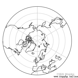
This is the bottom map of the map , We haven't drawn the data yet .
Average annual snow water equivalent mapping
swe=nc.Dataset('E:/arctic/XDA19070302_154/swe_year.nc')
lon=np.array(swe.variables['x'])
lat=np.array(swe.variables['y'])
swe_year=np.array(swe.variables['swe_year'])
# Import data
d=np.ma.masked_values(swe_year,-9999.0)
d=d/365# Average annual snow water equivalent
data_proj =ccrs.LambertAzimuthalEqualArea(central_latitude=90, central_longitude=0)# Set projection information of data , Pay attention to the original nc Projection information in the folder , Here is LambertAzimuthalEqualArea, The center longitude and latitude are 90°N,0°
c7=f1_ax1.pcolormesh(lon,lat,d,cmap=cmaps.BlAqGrYeOrRe,transform=data_proj,vmin=0,vmax=350)# Draw the annual average snow water equivalent
position=fig1.add_axes([0.2, 0.25, 0.55, 0.025])# Icon position
font = {
'family' : 'serif',
'color' : 'darkred',
'weight' : 'normal',
'size' : 16,
}
cb=fig1.colorbar(c7,cax=position,orientation='horizontal',format='%.1f',extend='both')# Set icon
cb.set_label('SWE(mm)',fontdict=font) # Add icon labels
#fig1.savefig('E:/arctic/2019SWE.jpg')# preservation
Last , A picture of the world :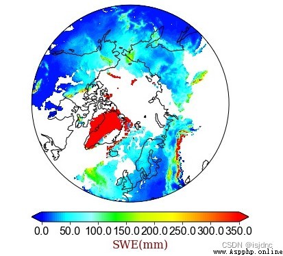
2019 The annual average snow water equivalent of the pan Arctic region in
Compare the data documents :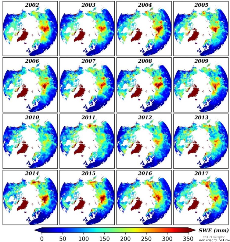
Integrated pan Arctic annual snow water equivalent (2002-2017 year )
The approximate distribution is correct , Specific drawing details can be set by yourself .
Color code
python The color code is not beautiful , There are great gods in the meteorological home NCL The color code of is moved to python in , The library is cmaps, What I use in drawing is the color code of this library , See cmaps
Add coordinates
Cartopy When drawing the polar projection itself bug, Because the boundary is square , When drawing , We're going to draw a circular boundary for it , At this time, longitude and latitude cannot be added , You can only roughly position yourself according to longitude and latitude , Add as text to the diagram , Add coordinates visible :
How to Add More Lines of Longitude/latitude in NorthPolarStereo Projection
I didn't add , Steal laziness ……
This nc The longitude and latitude of the data are XY Coordinate description , Although it has no effect on drawing , But considering the longitude and latitude coordinates, the setting of longitude and latitude is more intuitive and convenient , Here I post the code for converting this data coordinate :
import numpy as np
import math
'''
def XYtoGPS(x, y, ref_lat, ref_lon):
CONSTANTS_RADIUS_OF_EARTH = [6371000 for i in range(978)] # meters (m)
CONSTANTS_RADIUS_OF_EARTH=np.array(CONSTANTS_RADIUS_OF_EARTH,dtype=np.float32)
x_rad = np.divide(x,CONSTANTS_RADIUS_OF_EARTH)
y_rad = np.divide(x,CONSTANTS_RADIUS_OF_EARTH)
c = np.sqrt(x_rad * x_rad + y_rad * y_rad)
ref_lat_rad = np.radians(ref_lat)
ref_lon_rad = np.radians(ref_lon)
ref_sin_lat = np.sin(ref_lat_rad)
ref_cos_lat = np.cos(ref_lat_rad)
if abs(c) > 0:
sin_c = np.sin(c)
cos_c = np.cos(c)
lat_rad = np.asin(cos_c * ref_sin_lat + (x_rad * sin_c * ref_cos_lat) / c)
lon_rad = (ref_lon_rad + np.atan2(y_rad * sin_c, c * ref_cos_lat * cos_c - x_rad * ref_sin_lat * sin_c))
lat = np.degrees(lat_rad)
lon = np.degrees(lon_rad)
else:
lat = np.degrees(ref_lat)
lon = np.degrees(ref_lon)
return lat, lon
'''
ref_lat=[90 for i in range (978)]
ref_lon=[0 for i in range (978)]
CONSTANTS_RADIUS_OF_EARTH = [6371000 for i in range(978)] # meters (m)
CONSTANTS_RADIUS_OF_EARTH=np.array(CONSTANTS_RADIUS_OF_EARTH,dtype=np.float32)
x=lon
y=lat
x_rad =np.divide(x,CONSTANTS_RADIUS_OF_EARTH)
y_rad = np.divide(x,CONSTANTS_RADIUS_OF_EARTH)
c = np.sqrt(x_rad * x_rad + y_rad * y_rad)
ref_lat_rad = np.radians(ref_lat)
ref_lon_rad = np.radians(ref_lon)
lat1=[0 for i in range (978)]
lon1=[0 for i in range (978)]
ref_sin_lat = np.sin(ref_lat_rad)
ref_cos_lat = np.cos(ref_lat_rad)
A=np.arange(0,977,1)
for i in A:
if abs(c[i])>0:
sin_c = math.sin(c[i])
cos_c = math.cos(c[i])
lat_rad = math.asin(cos_c * ref_sin_lat[i] + (x_rad[i] * sin_c * ref_cos_lat[i]) / c[i])
lon_rad = (ref_lon_rad[i] + math.atan2(y_rad[i] * sin_c, c[i] * ref_cos_lat[i] * cos_c - x_rad[i] * ref_sin_lat[i] * sin_c))
lat1[i] = math.degrees(lat_rad)
lon1[i]= math.degrees(lon_rad)
else:
lat1[i] = math.degrees(ref_lat[i])
lon1[i]= math.degrees(ref_lon[i])
Data processing
python about nc Data processing , Personally, I feel that there is nothing wrong with it , be relative to Matlab and R for , Not much convenience , It's not too complicated , Data types are similar , actually , For any data processing , These languages are similar , As long as you master the common data types : list 、 Array 、 Dictionary, etc , Any language processing data is similar , Of course , Different languages will have some characteristic data types , such as matlab Of cell,R Data frame , However, the actual operation is not much different , Use whichever you are familiar with .
Drawing
My assessment is : Not as good as ArcGIS(×)
Icon settings and drawing size 、 The relative position setting is very cumbersome , The color matching is not very good , Drawing non equidistant color matching is troublesome , It's not as good as ArcGIS Intuitive and concise .
however ArcGIS It is a professional geographic information software , Perhaps there is no comparability .
if necessary ArcGIS mapping , It can be used gdal The library will nc To tif, And then GIS Middle drawing , But export as tif file matlav and R Can also do ……
Sum up ,python Handle nc And WRF The advantage of post-processing is : All gold language , You can download data at the same time 、 Processing data 、 mapping , It's more convenient .
however , Neither data processing nor drawing has any advantages , If you are used to it like me matlab and R Processing data , use ArcGIS If you plot , use python Don't have to , Instead, it will be because you are not familiar with debug Very long .
But it's no harm to run if you're free , As a simple programming reconstruction, it's still a little useful (×)
I may try it later if I am free GDAL Handle NC, Reuse GIS Draw a picture to compare .
Last , Attach complete code :
import numpy as np
import netCDF4 as nc
import matplotlib.pyplot as plt### Introducing library packages
import numpy as np
import matplotlib as mpl
import cartopy.crs as ccrs
import cartopy.feature as cfeature
from cartopy.mpl.gridliner import LONGITUDE_FORMATTER, LATITUDE_FORMATTER
import matplotlib.ticker as mticker
import netCDF4 as nc
import matplotlib.path as mpath
import cmaps
d=nc.Dataset('E:/arctic/XDA19070302_154/Arctic_SWE_2019.nc')
all_vars = d.variables.keys() # Get all variable names
all_vars_info = d.variables.items() # Get all variable information
print(type(all_vars_info)) # Output is : odict_items . Here it is translated into list list
all_vars_info = list(all_vars_info)
print(all_vars_info)
d_lon=np.array(d.variables['x'])
d_lat=np.array(d.variables['y'])
time=np.array(d.variables['time'])
d_lon=np.array(d.variables['x'])
d_lat=np.array(d.variables['y'])
swe=np.array(d.variables['swe'])
print("E's _FillValue are:")
FillValue_E=d.variables['swe']._FillValue
print(FillValue_E)
swe=np.ma.masked_values(swe,FillValue_E)
swe_year=np.transpose(np.sum(swe,axis=0))
swe_year=np.ma.filled(swe_year,FillValue_E)
f_w = nc.Dataset('E:/arctic/XDA19070302_154/swe_year.nc','w',format = 'NETCDF4') # Create a format of .nc Of , The name is ‘hecheng.nc’ The file of
f_w.createDimension('x',978)
f_w.createDimension('y',978)
f_w.createVariable('x',np.float32,('x'))
f_w.createVariable('y',np.float32,('y'))
f_w.variables['x'][:] = d_lon
f_w.variables['y'][:] = d_lat
f_w.createVariable( 'swe_year', np.float64, ('x','y'))
f_w.variables['swe_year'][:] = swe_year
f_w.close()
mpl.rcParams["font.family"] = 'Arial' # Default font type
mpl.rcParams["mathtext.fontset"] = 'cm' # Mathematical text font
mpl.rcParams["font.size"] = 16 # font size
mpl.rcParams["axes.linewidth"] = 1 # The thickness of the axis frame ( The default is too thick )
swe=nc.Dataset('E:/arctic/XDA19070302_154/swe_year.nc')
lon=np.array(swe.variables['x'])
lat=np.array(swe.variables['y'])
swe_year=np.array(swe.variables['swe_year'])
proj =ccrs.NorthPolarStereo(central_longitude=0)
# In cylindrical projection proj = ccrs.PlateCarree(central_longitude=xx)
leftlon, rightlon, lowerlat, upperlat = (-180,180,45,90)
# Draw only 60°E-90°E part
img_extent = [leftlon, rightlon, lowerlat, upperlat]
fig1 = plt.figure(figsize=(8,8))
f1_ax1 = fig1.add_axes([0.2, 0.3, 0.5, 0.5],projection = ccrs.NorthPolarStereo())
# Note that... Has been added here projection = ccrs.NorthPolarStereo(), Indicate the right to axes For the polar projection of the northern hemisphere
#f1_ax1.gridlines()
f1_ax1.set_extent(img_extent, ccrs.PlateCarree())
f1_ax1.add_feature(cfeature.COASTLINE.with_scale('110m'))
####### The following are the parameters of the grid line ######
theta = np.linspace(0, 2*np.pi, 100)
center, radius = [0.5, 0.5], 0.5
verts = np.vstack([np.sin(theta), np.cos(theta)]).T
circle = mpath.Path(verts * radius + center)
##############################
f1_ax1.set_boundary(circle, transform=f1_ax1.transAxes)
# Set up axes The border , Is a circular boundary , Otherwise, it is the polar projection of the square
d=np.ma.masked_values(swe_year,-9999.0)
d=d/365
#fig1.text(x, y, r'0$^\circ$',fontsize=14, horizontalalignment='center',verticalalignment='center')
data_proj =ccrs.LambertAzimuthalEqualArea(central_latitude=90, central_longitude=0)
c7=f1_ax1.pcolormesh(lon,lat,d,cmap=cmaps.BlAqGrYeOrRe,transform=data_proj,vmin=0,vmax=350)
#f1_ax1.contourf(lon,lat,swe_year, zorder=0, levels =np.arange(-0.6,0.7,0.1) , extend = 'both',transform=data_proj, cmap=plt.cm.RdBu_r)
position=fig1.add_axes([0.2, 0.25, 0.55, 0.025])
font = {
'family' : 'serif',
'color' : 'darkred',
'weight' : 'normal',
'size' : 16,
}
cb=fig1.colorbar(c7,cax=position,orientation='horizontal',format='%.1f',extend='both')
cb.set_label('SWE(mm)',fontdict=font)
#fig1.savefig('E:/arctic/2019SWE.jpg')