Similar to human eyes and brain ,OpenCV The main features of the image can be detected and this
Some features are extracted into the so-called image descriptor . then , These features can be used as data
library , Support image-based search . Besides , We can use key points to splice images
Come on , Form a larger image .( Imagine putting many pictures together to make one 360°
The panorama of .)
This chapter will show how to use OpenCV Detect the features in the image , And use these features
Match and retrieve images . In the learning process of this chapter , We will get the sample image and detect
Its main characteristics , Then try to find the area matching the sample image in another image .
We will also find the homography or space between the sample image and the matching area of another image
Relationship .
This chapter will introduce the following topics :
· Use any algorithm (Harris Corner point 、SIFT、SURF perhaps ORB) testing
Key points and extract local descriptors around key points .
· Use brute force algorithm or FLANN Algorithm matching key points .
· Use KNN And ratio test filter bad matching results .
· Find the homography between two groups of matching keys .
· Search for a set of images , Determine which image contains the best match of the reference image .
We're going to build a “ Concept – verification ” Judicial expertise application to complete
The content of this chapter . Given a reference image of tattoo , We will search for images of a group of people ,
In order to find out who matches the tattoo .
6.1 Technical requirements
It's used in this chapter Python、OpenCV as well as NumPy. About OpenCV, We used
Optional opencv_contrib modular , Including additional algorithms for key point detection and matching . want
Enable SIFT and SURF Algorithm ( Have a patent , Commercial use is not free ), We have to
CMake The configuration in has OPENCV_ENABLE_NONFREE logo opencv_contrib model
block . For installation instructions, refer to page 1 Chapter . Besides , If you haven't installed Matplotlib, can
To run $ pip install matplotlib( or $ pip3 install matplotlib,
It depends on the environment ) install Matplotlib.
The complete code of this chapter can be found in GitHub library
(https://github.com/PacktPublishing/Learning-OpenCV-4-
Computer-Vision-with-Python-Third-Edition) Of chapter06 Folder
Find . Example images can be found in images Found in folder .
6.2 Understand the types of feature detection and matching
There are many algorithms that can be used to detect and describe features , This section will explore some of these calculations
Law .OpenCV The most commonly used feature detection and descriptor extraction algorithms are as follows :
·Harris: This algorithm is suitable for corner detection .
·SIFT: This algorithm is suitable for spot detection .
·SURF: This algorithm is suitable for spot detection .
·FAST: This algorithm is suitable for corner detection .
·BRIEF: This algorithm is suitable for spot detection .
·ORB: It is Oriented FAST and Rotated BRIEF The joint abbreviation of .ORB Yes
It is very useful for the combined detection of corners and spots .
The following methods can be used for feature matching :
· Brute force match .
· be based on FLANN The matching of .
Spatial verification can be carried out through homography .
We have just introduced many new terms and algorithms . Now? , Let's discuss their
The basic definition .
Feature definition
What are the characteristics ? Why can a specific area of an image be classified as a feature ,
Other areas cannot be classified as features ? Broadly speaking , Features are unique or contained in the image
An easily recognizable region of interest . Corners and areas with high density texture detail are good
features , In low-density areas ( Like blue sky ) Repeated patterns are not good characteristics
sign . Edge is a good feature , Because they tend to divide the image into two regions . speckle
( Image area that is very different from the surrounding area ) It is also an interesting feature .
Most feature detection algorithms revolve around corners 、 The recognition of edges and spots unfolds , Yes
Some people also pay attention to the mountains (ridge) The concept of , Ridge can be conceptualized as symmetry of slender objects
Axis .( for example , Imagine recognizing a road in an image .)
Some algorithms are better at recognizing and extracting specific types of features , So understand the input image
What is important , In this way, we can make use of OpenCV The best tool in .
6.3 testing Harris Corner point
Let's start with Harris Corner detection algorithm . We use an example to complete the corner
Point detection task . If you are after reading this tutorial , Continue to study OpenCV, Then you will
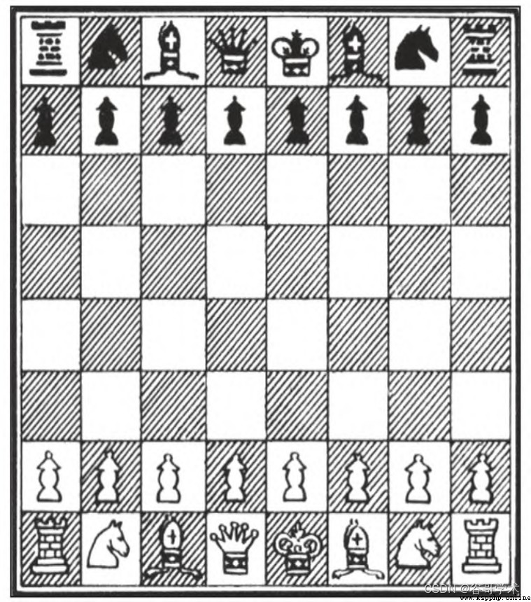
Finding checkerboard is a common subject of computer vision analysis , Part of the reason is that the chessboard mode is suitable
Used for many types of feature detection , Part of the reason is that playing chess is a popular pastime
type , Especially in Russia —— There are many OpenCV Developer .
chart 6-1 Is an example image of a chessboard and pieces .
OpenCV There is one named cv2.cornerHarris Convenient function of , Used to detect images
Corner of . In the following basic example , We can take a look at the operation of this function
condition :

Let's analyze the code . After general import , Load the chessboard image and convert it
Grayscale image . Next , call cornerHarris function :
The most important parameter here is number 3 Parameters , Defines Sobel (Sobel) Operator's
Aperture or core size . Sobel operator measures the horizontal and vertical differences between the pixel values in the neighborhood
Different to detect edges , And use the core to achieve this task .cv2.cornerHarris Function to make
The aperture of the Sobel operator used is defined by this parameter . In short , These parameters define the angle
Sensitivity of point detection . This parameter value must be in 3~31 Odd values between . about 3 this
Kind of low value ( High sensitivity ), All slashes in the black square on the chessboard touch the border of the square
when , Will be recorded as corners . about 23 Such high value ( Low sensitivity ), Only everyone
The corners of the lattice will be detected as corners .
cv2.cornerHarris Returns an image in floating-point format . Each value in the image represents
A score of the corresponding pixel of the source image . A medium or high score indicates that the pixel is very good
It can be a corner . contrary , The pixel with the lowest score can be regarded as a non corner . Consider the following
Lines of code :

here , The score of the pixel we select is at least the highest 1%, And in the original figure
Paint these pixels red , The result is shown in Fig. 6-2 Shown .
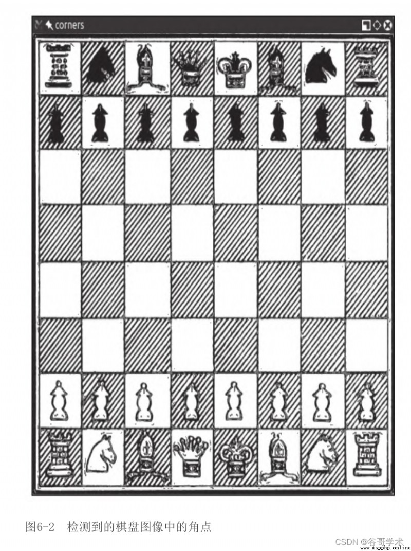
fantastic ! Almost all detected corners are marked in red . The marked points include chess
Almost all corners on the grid .
If you adjust cv2.cornerHarris No 2 Parameters , We will see smaller
Area ( Corresponding to smaller parameter values ) Or a larger area ( Corresponding to larger parameters
value ) Detected as corners . This parameter is called the block size .
6.4 testing DoG Feature and extract SIFT The descriptor
The above technology uses cv2.cornerHarris, It can detect corners well and has obvious
advantage , Because the corner is the corner , These corners can be detected even if the image is rotated . however ,
If you zoom the image to a smaller or larger size , Some parts of the image may be missing or
Get high-quality corners .
for example , chart 6-3 yes F1 Corner detection results of an image of the Italian Grand Prix track .
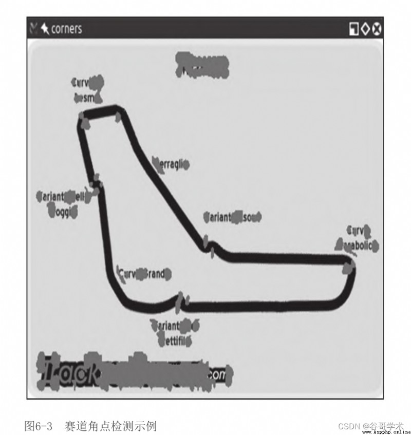
chart 6-4 It is a smaller version of corner detection results based on the same image
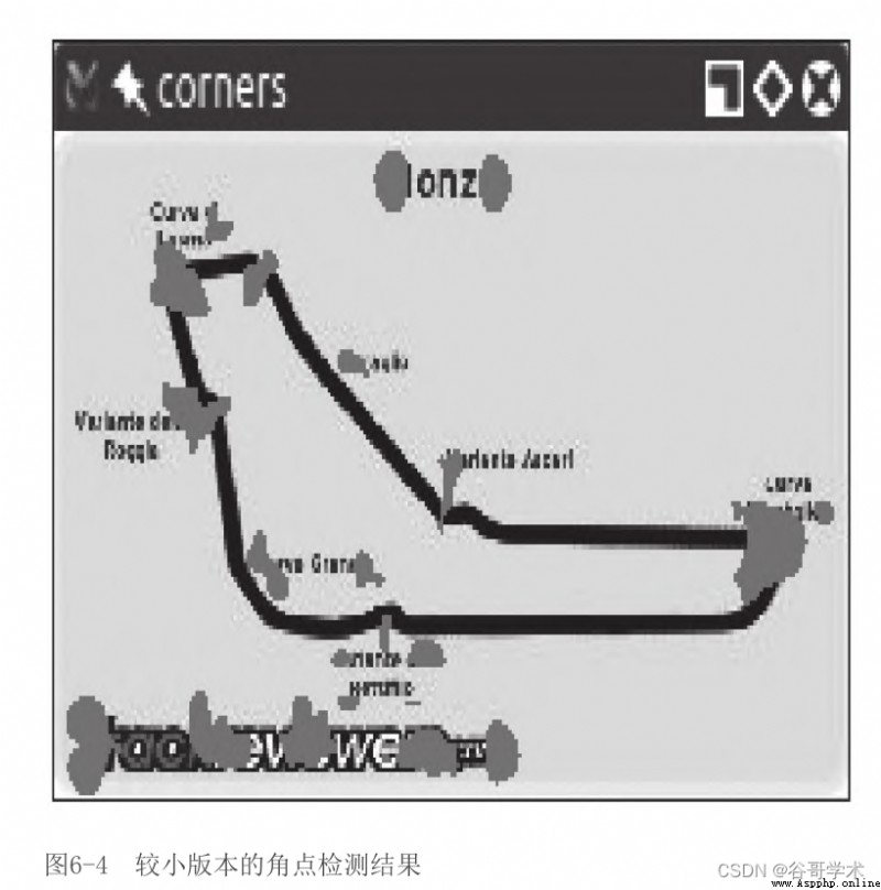
You will notice how the corners become more compact , But , Although we got a
Some corners , But also lost some corners ! such as , Let's check askari
(Variante Ascari) Deceleration curve , This track is located at the end of the track from northwest to Southeast
The curve of looks like a wavy curve . In the large version of the image , The entrance and top of the double bend
Are detected as corners . In a reduced version of the image , No such top was detected . Such as
If you further reduce the image , To some extent, we will also lose the corner of the curve entrance .
The loss of this feature raises a problem : We need an algorithm , No matter the image
Size can work . So scale invariant feature transformation (Scale-Invariant Feature
Transform,SIFT) Debut . Although the name sounds a little mysterious , But since
We know what problem to solve , It is actually meaningful . We need a
function ( Transformation ) To detect features ( Feature change ), And it won't vary with the image scale
And output different results ( Scale invariant feature transformation ). Please note that ,SIFT Do not detect key
spot ( Use Gauss difference (Difference of Gaussian,DoG) To complete ), But through
Describe the region around it by eigenvectors .
Next, take a quick look DoG. In the 3 In the chapter , We discuss low pass filters and
Fuzzy operation , especially cv2.GaussianBlur() function .DoG It is the application of the same image
Results of different Gaussian filters . Before , We apply this kind of technology to edge detection ,
The idea here is the same .DoG The final result of the operation contains the region of interest ( Key points ),
And then through SIFT Describe .
Let's see DoG and SIFT In the figure 6-5 Performance in , This image is full of corners and features
sign .
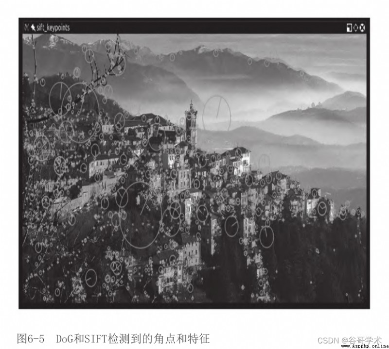
Valez is used here ( Located in Lombardy, Italy ) Beautiful panorama of , This figure
In the field of computer vision, it is famous as a subject . The following is the generated processed
Image code :
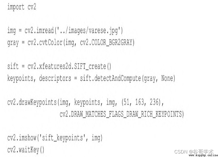
After general import , Load the image you want to process . then , Convert the image into a grayscale image
image . thus , You may have found out OpenCV Many methods in need of gray image as
Input . The next step is to create SIFT Test object , And calculate the characteristics and description of gray image
operator :
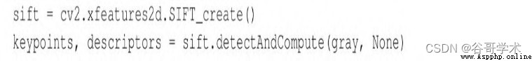
Backstage , These simple lines of code perform a complex process : Create a
cv2.SIFT object , This object uses DoG Detect key points , Then calculate the area around each key
The eigenvector of the field . just as detectAndCompute The name of the method clearly indicates that ,
This method mainly performs two operations : Feature detection and descriptor calculation . The return value of this operation
It's a tuple , Contains a list of keys and a list of descriptors for another key .
Last , use cv2.drawKeypoints Function to draw keys on the image , Then use regular
Regular cv2.imshow Function to display it . As one of the parameters ,
cv2.drawKeypoints The function accepts a flag that specifies the type of visualization you want . this
in , We specify cv2.DRAW_MATCHES_FLAGS_DRAW_RICH_KEYPOINT, In order to draw
Make the visualization of the scale and direction of each key point .
Analysis of key points
Every key point is cv2.KeyPoint An instance of a class , Has the following properties :
·pt( spot ) Attributes include key points in the image x and y coordinate .
·size The attribute represents the diameter of the feature .
·angle The attribute represents the direction of the feature , As shown by the radial line in the previously processed image
in .
·response The attribute represents the strength of the key . from SIFT Some features of classification are better than others
Stronger features ,response Feature strength can be evaluated .
·octave Attribute represents the image pyramid layer where the feature is found . Let's briefly review
5.2 The concept of image pyramid introduced in section .SIFT The operation of the algorithm is similar to face
Detection algorithm , Iteratively process the same image , But the input changes every iteration . have
Physically speaking , The image scale is in each iteration of the algorithm (octave) A parameter that changes over time .
therefore ,octave Attributes are related to the image scale of the detected key points .
·class_id Attributes can be used to assign custom to a key or a group of keys
Identifier .
6.5 Fast detection Hessian Feature and extract SURF The descriptor
Computer vision is a relatively new branch of Computer Science , So many famous
The algorithm and technology of are all recent . actually ,SIFT Is in 1999 Year by year David
Lowe released , Only 20 Years of history .
SURF Is in 2006 Year by year Herbert Bay Released a feature detection algorithm .SURF want
Than SIFT How fast , And it was SIFT Inspired by the .
Please note that ,SIFT and SURF Are authorized patent algorithms , therefore , Only in
opencv_contrib構建 in Use 了OPENCV_ENABLE_NONFREE CMake mark
Only when you are ready .
For this tutorial , understand SURF The working principle of is not particularly important , We can
Apply it to the application and make full use of it . It's important to understand cv2.SURF
It's a OpenCV class , Use fast Hessian Algorithm for key point detection , And use SURF Conduct
Descriptor extraction , It's like cv2.SIFT Similar to class ( use DoG Carry out key point detection , use SIFT Into the
Row descriptor extraction ).
Besides , The good news is OpenCV All feature detection and descriptor extraction supported by it
The algorithm provides a standard API. therefore , Just make some minor changes , I can modify it
The previous code example uses SURF( instead of SIFT). Here is the modified code ,
The modified part is shown in bold :
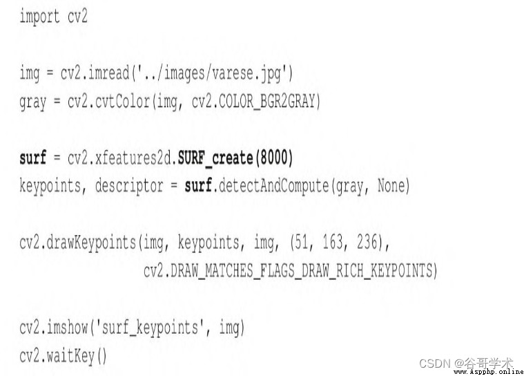
cv2.xfeatures2d.SURF_create The parameter of is fast Hessian One of the algorithms
threshold . By increasing the threshold , It can reduce the number of retained features . The threshold for 8000
when , The results are shown in the figure 6-6 Shown .
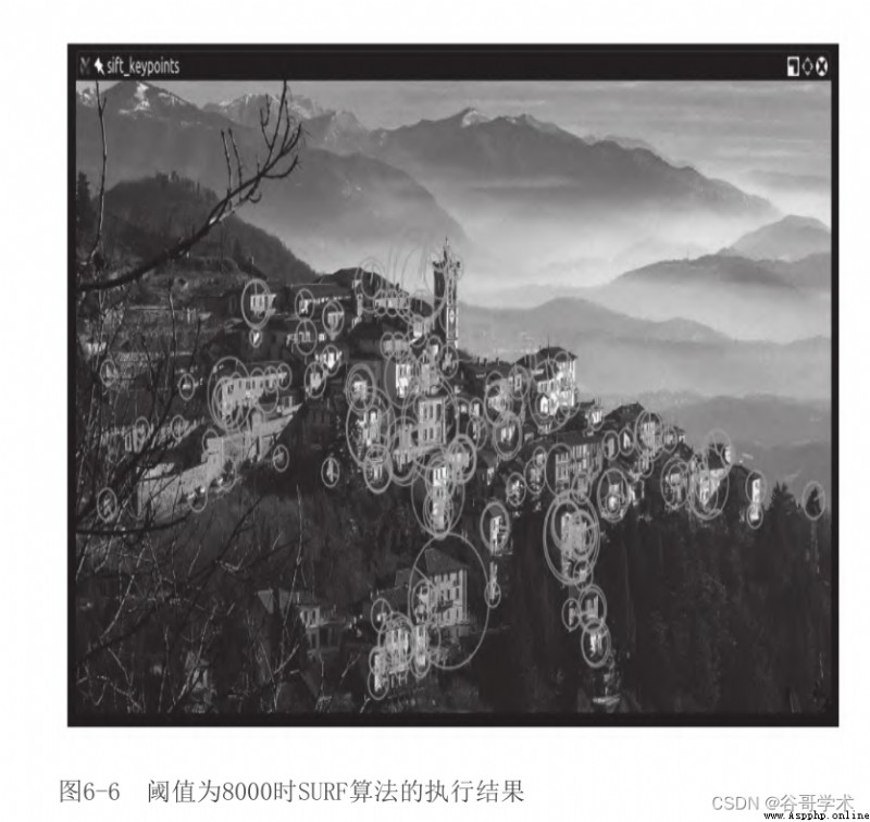
Try adjusting the threshold , Look at the impact of the threshold on the results . As a practice , You may wish
Build a slider with a control threshold GUI Applications . In this way , Users can adjust
Integer threshold , See the number of features that increase and decrease in inverse proportion . stay 4.7 In the festival , We
Built a with slider GUI Applications , So you can refer to that part .
Next , We will study FAST Corner detector 、BRIEF Key descriptor and
ORB( hold FAST and BRIEF To use together ).
6.6 Using a FAST The characteristics and BRIEF Descriptors ORB
if SIFT Still very young ,SURF Younger , that ORB Is still in infancy .
ORB First published in 2011 year , As SIFT and SURF A quick substitute for .
The algorithm is published in the paper “ORB:an efficient alternative to SIFT or
SURF” On , Can be in
http://www.willowgarage.com/sites/default/files/orb_final.pdf
Found at PDF The format of the paper .
ORB Integrated FAST Key point detector and BRIEF Key descriptors , So it's necessary to
So let's see FAST and BRIEF. Next , We will discuss brute force matching ( Used for feature matching
Matching algorithm ) And give an example of feature matching .
6.6.1 FAST
Features of accelerated segmentation testing (Feature from Accelerated Segment
Test,FAST) The algorithm is through analysis 16 A circular neighborhood of pixels .FAST count
Method marks each pixel in the neighborhood as brighter or darker than the bit threshold , This threshold is relative to
Defined by the center of the circle . If the neighborhood contains a series of continuous images marked brighter or darker
plain , Then this neighborhood is regarded as a corner .
FAST A high-speed test is also used , Sometimes you can just check 2 A or 4 Like
plain ( instead of 16 Pixel ) To make sure that the neighborhood is not a corner . To understand how this test works
do , Let's take a look at the picture below 6-7( selected from OpenCV file ).
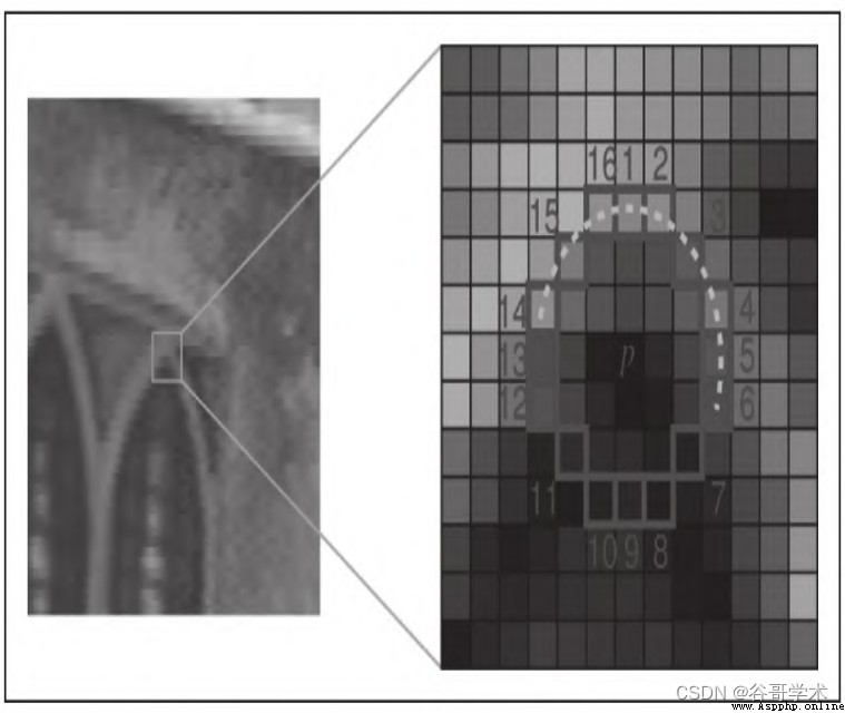
In the figure 6-7 Under two different magnification , We can see a 16 Adjacent to pixels
Domain . be located 1、5、9 and 13 The pixel at corresponds to the edge of the circular neighborhood 4 Four cardinal points .
If the neighborhood is a corner , Then it is expected to be here 4 In pixels , There's just 3 Pixels or 1
Pixels are brighter than the threshold .( Another saying is that there happens to be 1 A or 3 Pixel ratio threshold
dark .) If there happens to be 2 One is brighter than the threshold , Then this field is one side , Rather than one
Corner points . If there happens to be 4 A or 0 One is brighter than the threshold , Then this field is relatively one
Cause , Neither corner nor edge .
FAST It is an intelligent algorithm , But it is not without shortcomings , To make up for these deficiencies
spot , Developers engaged in image analysis can implement a machine learning algorithm , In order to calculate
Method provides a set ( Related to a given application ) Images , So as to optimize parameters such as threshold .
Whether the developer directly specifies parameters , Or provide a training for machine learning methods
Set ,FAST It is an algorithm that is very sensitive to input , Maybe more than SIFT More sensitive .
6.6.2 BRIEF
in addition , Basic characteristics of binary robust independence (Binary Robust Independent
Elementary Feature,BRIEF) Not a feature detection algorithm , It's a descriptor .
Let's take a closer look at the concept of descriptors , Then study BRIEF.
Use... In the front SIFT and SURF When analyzing images , The core of the whole process is to call
detectAndCompute function . This function performs two different steps —— Detection and measurement
count , They return to 2 Different results ( Coupled to a tuple ).
The test result is a set of key points , The result is a set of descriptors for these key points .
It means OpenCV Of cv2.SIFT and cv2.SURF Classes implement detection and description algorithms .
please remember , The original SIFT and SURF Not a feature detection algorithm .OpenCV Of cv2.SIFT real
Now DoG Feature detection and SIFT describe , and OpenCV Of cv2.SURF Fast
Hessian Feature detection and SURF describe .
Key descriptor is a representation of image , Act as a channel for feature matching , Because of you
You can compare the key descriptors of two images and find their commonalities .
BRIEF It is one of the fastest descriptors at present .BRIEF The theory behind it is quite complicated , but
It can be said that ,BRIEF Adopt a series of optimization , Make it a very important feature matching
Good choice .
6.6.3 Brute force match
Brute force matcher is a descriptor matcher , It compares the juxtaposition of two sets of key descriptors
Into a matching list . It is called brute force matching , It is because there is almost no optimization involved in this algorithm
turn . For each key descriptor in the first set , The matcher matches it with the second set
Compare each key descriptor in the combination . Each comparison produces a distance value , Dyadic
Choose the best match at the minimum distance .
In a nutshell , In calculation ,“ sheer animal strength ” The word "combination" refers to the combination of all possible ( example
Such as , Crack all possible character combinations of passwords of known length ) The list of is sorted by priority
Methods . contrary , Algorithms that prioritize speed may skip some possibilities , And try to
Take a shortcut to find the most reasonable solution .
OpenCV Provides a cv2.BFMatcher class , Support several brute force feature matching methods
Law .
6.6.4 Match the logo in the two images
Now that we have a general understanding of what is FAST and BRIEF, We can understand it as
what ORB The team behind ( from Ethan Rublee、Vincent Rabaud、Kurt
Konolige and Gary R.Bradski form ) Choose these two algorithms as ORB The foundation of .
In his paper , The author's goal is to achieve the following results :
· by FAST Add a quick and accurate positioning component .
· oriented BRIEF Efficient calculation of features .
· oriented BRIEF Variance and correlation analysis of features .
· In terms of rotation invariance BRIEF A learning method of characteristics , In the nearest neighbor
Better performance in use .
The point is clear :ORB Our goal is to optimize and accelerate operations , Including the very important spin
Use the way of perception BRIEF Steps for , In this way, matching can be improved , Even in the training chart
The same is true when there is a very different rotation state from the query image .
however , At this stage , You may already know enough theory , Hope to further study
Study some feature matching , Let's look at some code . The following script attempts to put the special in the logo
The feature matches the feature in the photo containing the logo :
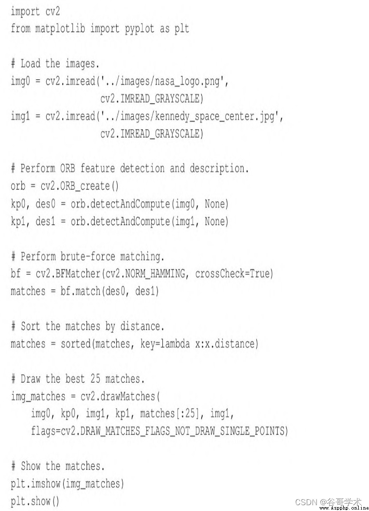
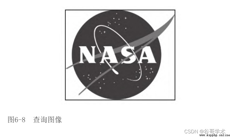
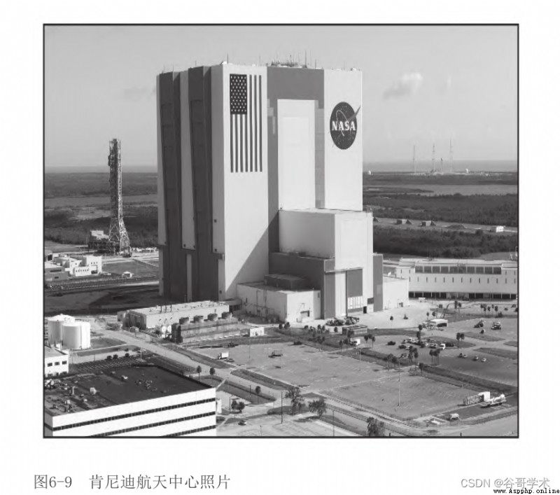
Let's look at this code step by step . After the usual import statement , We use
Load two images in grayscale format ( Query images and scenes ). chart 6-8 Is to query the image , It is
NASA logo . chart 6-9 It's a picture of Kennedy Space Center .
Now? , We continue to create ORB Feature detectors and descriptors :
 And use SIFT and SURF In a similar way , We detect and calculate the correlation between these two images
Key points and descriptors .
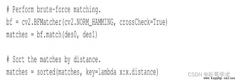
So let's start here , The concept is very simple : Traverse the descriptor and determine whether it matches , then
Calculate the matching mass ( distance ), And sort the matches , In this way, you can
Before the degree display n A match , They actually match the features on the two images .
cv2.BFMatcher It can be done :
At this stage , We have all the information we need , But as computer vision
lovers , We attach great importance to the visual representation of data , So we are matplotlib chart
Draw these matches in the table :
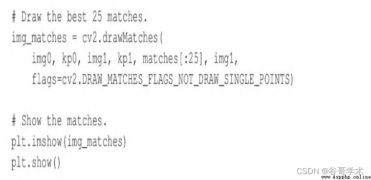
Python The slicing syntax of is very robust . If matches The list contains fewer items
On 25 individual , that matches[:25] The slice command will run normally , And provide with the original list containing
The same multi-element list .
The matching result is shown in the figure 6-10 Shown .
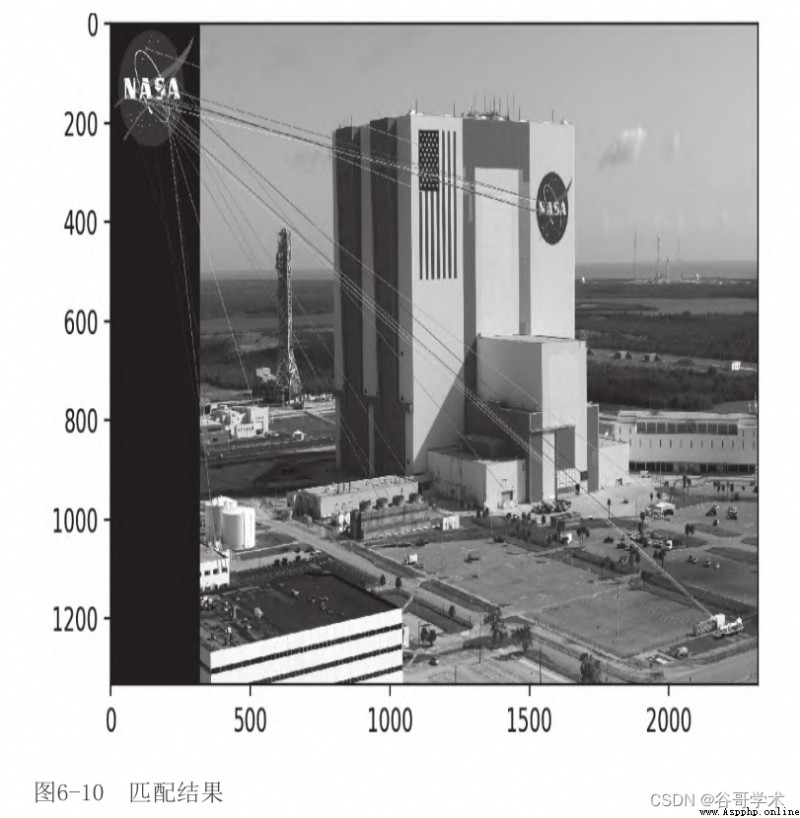
You may think this is a disappointing result . actually , We can see
Most matches are false . Unfortunately , It's typical . In order to improve the matching results ,
We need to apply other techniques to filter bad matches . Next we will turn our attention to
To this task .
6.7 Use K Nearest neighbor sum ratio test filter match
Imagine , A large group of well-known philosophers invite you to judge them about life 、 The universe
And everything is important to a debate . When each philosopher takes turns speaking ,
You will listen carefully . Last , When all philosophers have published all their arguments , you
Browsing notes , You will find the following two things :
· Every philosopher doesn't agree with other philosophers .
· No philosopher is more persuasive than other philosophers .
According to the initial observation , You infer that at most one philosopher is right ,
But in fact , It is also possible that all philosophers are wrong . then , According to the second
Secondary observation , Even if one of the philosophers is right , You will also start to worry about the possibility
Will choose a philosopher with a wrong view . No matter what you think , These people will make you late
Late for dinner . You call it a draw , And said that the most important issues in the debate remain unresolved .
We can judge whether the hypothetical problems debated by philosophers match the key points of poor filtering
Compare actual problems .
First , Suppose that at most one key point in the query image is correct
matching . in other words , If the query image is NASA identification , Then suppose another image
( scene ) Contains at most one NASA identification . Suppose a query key has at most one positive
An exact or good match , So when considering all possible matches , We mainly observe bad
Cake matching . therefore , The brute force matcher calculates the distance score of each possible match , It can be mentioned
For a large number of observations on the distance score of poor matching . Compared with countless bad matches , I
We hope that a good match will be significantly better ( A lower ) Distance score of , So bad horse
The score value can help us choose a threshold for a good match . Such a threshold is not
It must be well extended to different query key points or different scenarios , But at least
Specific cases will be helpful .
Now? , Let's consider the implementation of the modified brute force matching algorithm , The algorithm is based on the above
Way to adaptively select the distance threshold . In the example code in the previous section , We use
cv2.BFMatcher Class match Method to get a single best
matching ( Minimum distance ) A list of . Such an implementation discards all possible bad matches
Information about the assigned distance score , This kind of information is needed by adaptive methods . lucky
yes ,cv2.BFMatcher It also provides knnMatch Method , This method takes a parameter k,
You can specify the best that you want to keep for each query key ( Shortest distance ) The maximum number of matches
Number .( In some cases , The number of matches obtained may be greater than the specified maximum number
Less .)KNN Express K Nearest neighbor (K-Nearest Neighbor).
We will use knnMatch Method requests two best matches for each query key
list . Based on the assumption that there is at most one correct match for each query key , We are convinced that
Excellent matching is wrong . Multiply the distance score of suboptimal matching by a less than 1 Value , You can get
Threshold .
then , Only when the distance score is less than the threshold , Just regard the best match as a good match
with . This method is called ratio test (ratio test), First of all by David
Lowe(SIFT The author of the algorithm ) Bring up the . He's in a paper “Distinctive Image
Features from Scale-Invariant Keypoints”( The website is
https://www.cs.ubc.cs/~lowe/papers/ijcv04.pdf) Ratio checking is described in
Examination . say concretely , stay “Application to object recognition” part , He
The statement is as follows :
The probability of a correct match can be based on the nearest neighbor to the 2 The distance ratio of the nearest neighbor is accurate
set .
We can load the image in the same way as the previous code example 、 Detect key points ,
And calculate ORB The descriptor . then , Use the following two lines of code to perform brute force KNN matching :
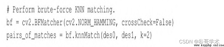
knnMatch Return the list of lists , Each internal list contains at least one match ,
And no more than k Matches , Each match from the best ( Shortest distance ) To the worst .
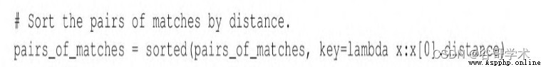
The following code line sorts the external list according to the distance score of the best match :
Let's draw the front 25 A perfect match , as well as knnMatch All that may be paired with it
Suboptimal matching . Out of commission cv2.drawMatches function , Because this function only accepts one-dimensional matches
Matching list , contrary , You have to use cv2.drawMatchesKnn. The following code is used to select
Choose 、 draw , And display the match :
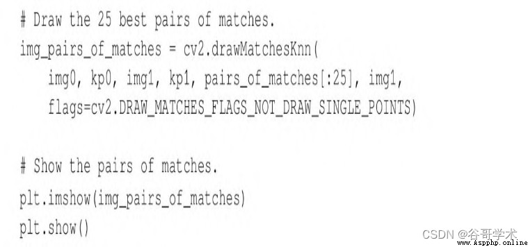
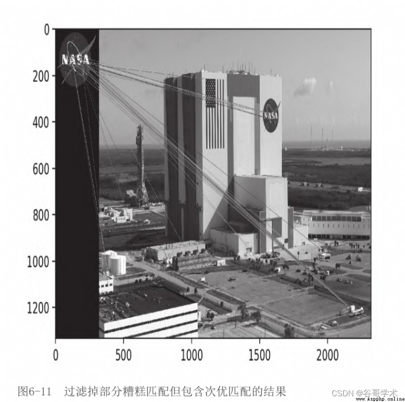
up to now , We haven't filtered out all the bad matches yet —— actually , also
Deliberately contains what we think is a bad sub optimal match —— therefore , The result looks a little
The disorderly , Pictured 6-11 Shown .
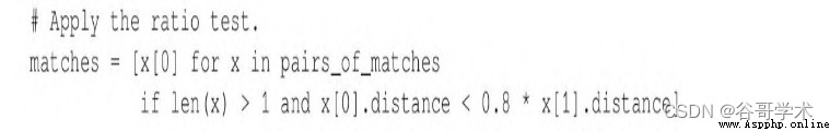
Now? , Let's apply the ratio test , Set the threshold value to... Of the sub optimal matching distance score
0.8 times . If knnMatch Cannot provide a suboptimal match , Then reject the best match , because
Cannot apply inspection to it . The following code applies these conditions , And provide tested
Best bet list :
After applying the ratio test , Just deal with the best match ( Not the best and suboptimal match
Yes ), In this way, you can use cv2.drawMatches( Instead of cv2.drawMatchesKnn) Yes
It is drawn . Again , Select front... From the list 25 Matches . The following code is used to select
Choose 、 draw , And display the matches :
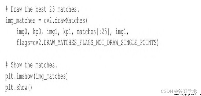
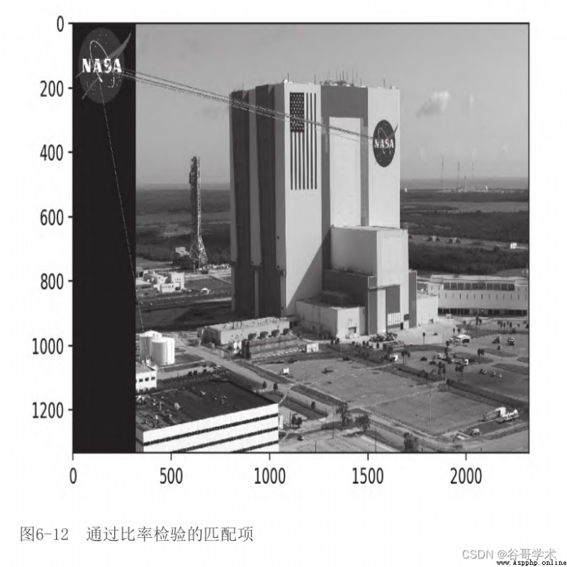
In the figure 6-12 in , We can see the matching items that pass the ratio test .
Compare this output image with the output image in the previous section , You can see the use of KNN
And ratio test can filter out many bad matches . The remaining matches are not perfect ,
But almost all matches point to the right area —— On the side of Kennedy Space Center
Of NASA identification .
We have a good start . Next , We will use the name FLANN Faster
The matcher replaces the brute force matcher . After that , We will learn how to trace according to homography
Describe a set of matches , That is, the position of the matching object 、 Rotation Angle 、 Scale and other geometry
Two dimensional transformation matrix of features .
6.8 be based on FLANN The matching of
FLANN Represents fast approximate nearest neighbor Library (Fast Library for Approximate
Nearest Neighbor), yes 2 Clause BSD An open source library under license .FLANN The official
Website is http://www.cs.ubc.ca/research/flann/. The following is excerpted from this website
standing :
FLANN It is a library that performs fast approximate nearest neighbor search in high-dimensional space , Contains the most
An algorithm set suitable for nearest neighbor search , And automatically select the best algorithm and
A system of optimal parameters .
FLANN Yes, it is C++ Compiling , contain C、MATLAB and Python Such as language binding
set .
Or say ,FLANN There is a big toolbox , Know how to choose a good one according to the task
Tools , And can speak several languages . These features make the library more convenient 、 quick . in fact ,FLANN
The author claims that : For many datasets ,FLANN Faster than other nearest neighbor search software
10 times .
As a separate library ,FLANN Can be in GitHub platform
(https://github.com/mariusmuja/flann/) Found on the . however , We will
take FLANN As OpenCV Part of the , because OpenCV It provides a convenience
The package of .
To start FLANN Actual examples of matching , Import first NumPy、OpenCV and
Matplotlib, And load two images from the file . Here's the code :
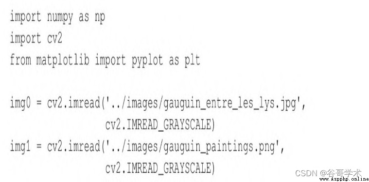
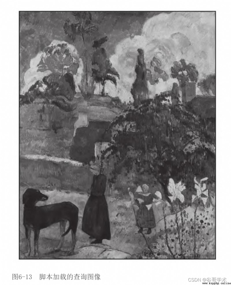
chart 6-13 Is the first image loaded by the script ( Query image ).
This work of art is Paul · gauguin (Paul Gauguin) On 1889 Completed in
Of Entre les lys(Among the lilies). We will include several Gauguin works
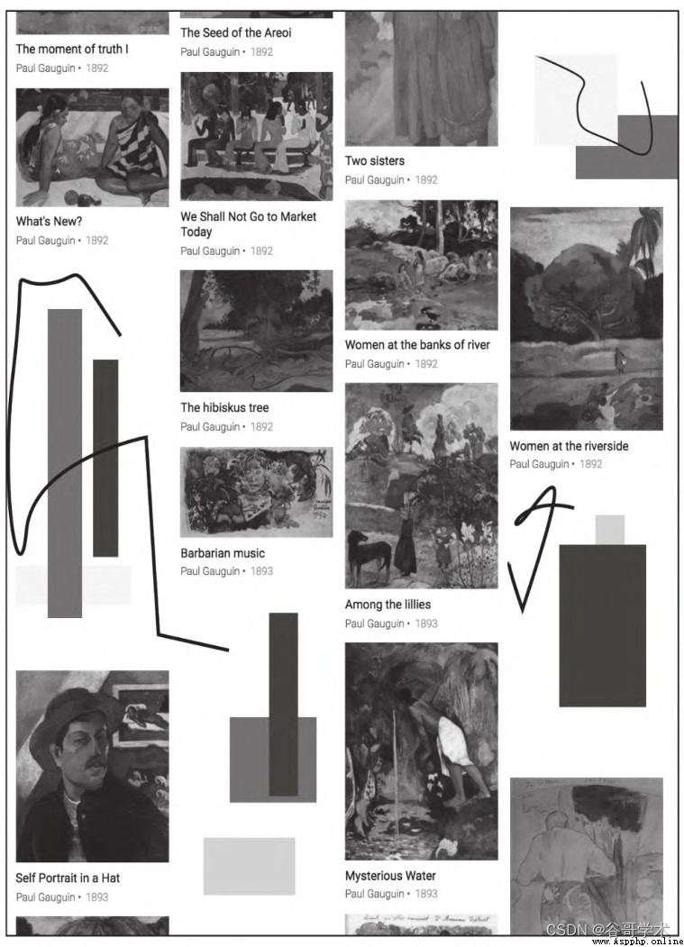
And some larger images with arbitrary shapes drawn by an author of this tutorial ( See the picture 6-14) Middle search
Match key points with cables .
In the big picture ,Entre les lys Located at 3 Xing di 3 Column . Query image and large image
The corresponding areas in are inconsistent , They are depicted in slightly different colors and different scales Entre
les lys. For all that , For our matcher , This should be a relatively simple
The situation of .
We use cv2.SIFT Class to detect the necessary key points , And extract features :
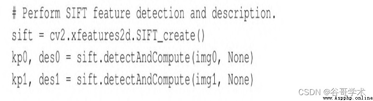
up to now , The code should look familiar , Because the previous sections of this chapter have been devoted to
Discussed SIFT And other descriptors . In the previous example , We send the descriptor into
cv2.BFMatcher, For brute force matching . This time, , We will use
cv2.FlannBasedMatcher. The following code uses custom parameters to execute based on FLANN Of
matching :
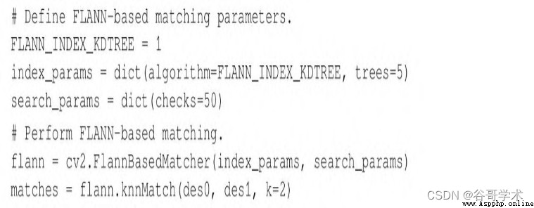
You can see ,FLANN The matcher accepts 2 Parameters :indexParams Objects and
searchParams object . These parameters are Python Chinese Dictionary ( and C++ Middle structure ) The shape of
Pass through , determine FLANN Internal behavior used to calculate the matching index and search objects . We
The selected parameters provide a reasonable balance between accuracy and processing speed . say concretely , We
Include is used 5 The nuclear density of a tree (kernel density tree,kd-tree) Indexes
Algorithm ,FLANN This algorithm can be processed in parallel .FLANN The document is suggested in 1 tree ( Not available and
Workability ) and 16 tree ( If the system can be used , Then you can provide a high degree of and
Workability ) Choose between .
We execute for each tree 50 Check or traverse times . The more times you check , Can provide
The higher the accuracy of , But the calculation cost is higher .
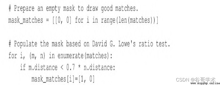
Based on FLANN After the match of , We apply a multiplier of 0.7 Lloyd's ratio test
Examination . To show different coding styles , Compared with the code example in the previous section , We're going to
The results of the ratio test are used in a slightly different way . Before , We have formed a new
A list of , It only contains good matches . This time, , We will form a group called
mask_matches A list of , Each of these elements is of length k( And pass on to knnMatch Of
k It's the same ) A sublist of . If the match is successful , Then set the corresponding element in the sub list to
1, Otherwise, set it to 0.
for example , If mask_matches=[[0,0],[1,0]], This means that there are two matches
The key point of : For the first key point , The best and suboptimal matches are bad ; And yes
In the second key point , The best match is good , Suboptimal matching is bad . Please note that , I
We assume that all suboptimal matches are bad . Use the following code to apply the ratio test ,
And create a mask :
Now is the time to draw and display good matches . hold mask_matches List transmission
hand cv2.drawMatchesKnn As an optional parameter , As shown in bold in the following code snippet :
cv2.drawMatchesKnn Only draw matches marked as good in the mask ( The value is 1). foot
This generated is based on FLANN The matching visualization results are shown in the figure 6-15 Shown .
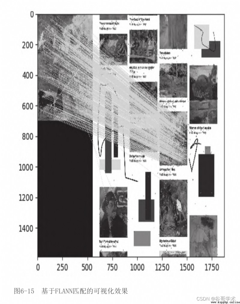
The results are encouraging : It seems that almost all matches are in the right position . Pick up
Come down , We try to simplify this type of result into a more concise geometric representation —— List should be
sex , It will describe the posture of the whole matching object , Instead of a bunch of discontinuous matching points .
6.9 be based on FLANN Homography matching
First , What is homography (homography)? One definition from the network is :
A relationship between two graphs , Any point of a graph and a point of another graph
Corresponding , vice versa . therefore , A tangent rolling on the circle cuts the two fixed tangents of the circle
Cut the line into two groups of isomorphic dots .
If you, like the author of this tutorial, don't know the previous definition , You might notice
The following explanation may be clearer : Homography is when one graph is a permutation of another graph
Visual distortion , Look for a situation of each other in the two pictures .
First , Let's see what we want to achieve , In this way, we can fully understand what is simple
sex . then , Check the code again .
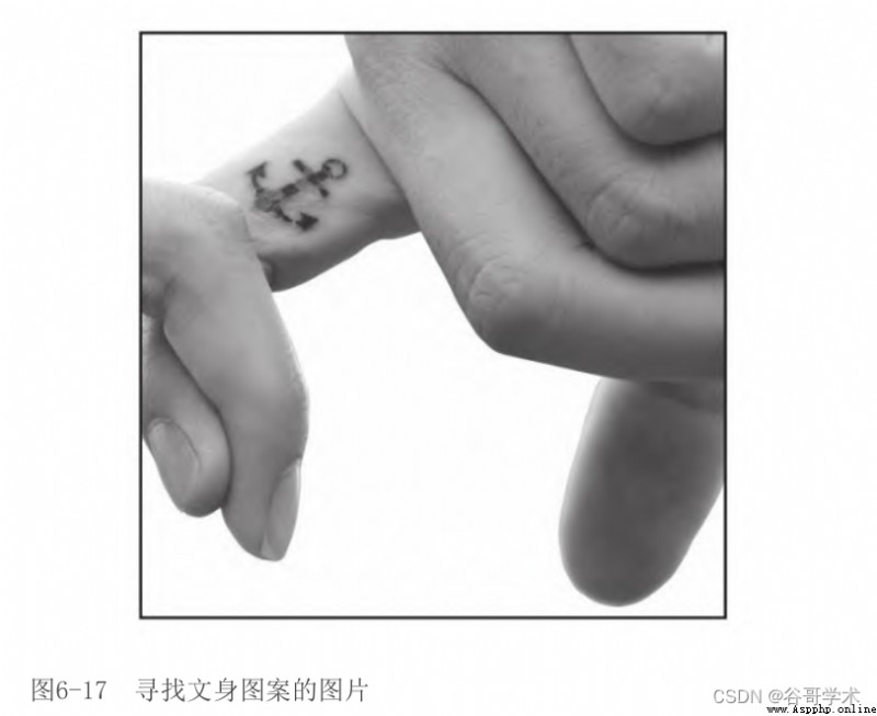
hypothesis , We want to search the map 6-16 Tattoo in .
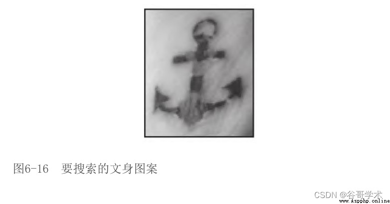
For us , It's easy to figure 6-17 Found tattoos in , Although there are some spins
The difference in angle .
As an exercise in the field of computer vision , We want to write a script to generate
Next key point matching and homography visualization results , Pictured 6-18 Shown .
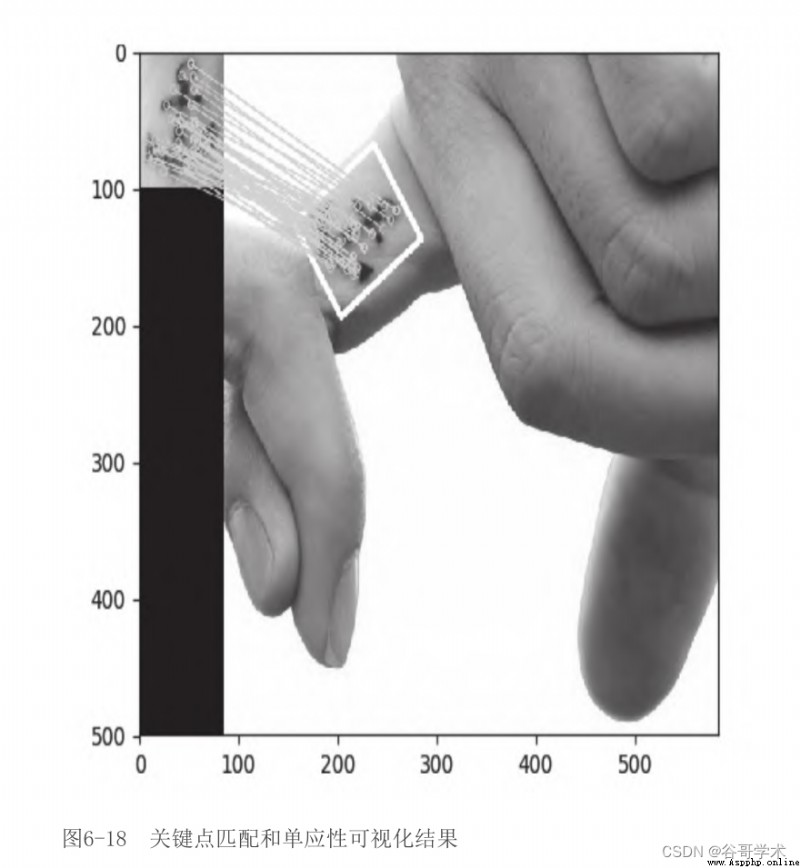
In the figure 6-18 in , We selected the main body in the first picture , Correct in the second picture
Identify the subject , Match lines are drawn between the keys , Even in the second picture
A white border , Show the body perspective distortion relative to the first image .
You may have guessed , The implementation of script starts from importing Library , Read grayscale format
Images , Detect features and calculate SIFT The descriptor . We have done all of the above in the previous example
There are these things , So I won't repeat it here . Let's see what to do next !
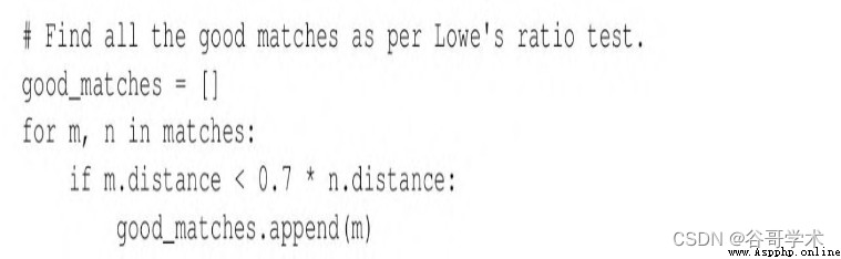
(1) We build a matching list that has passed the Lloyd's ratio test , The code is as follows :
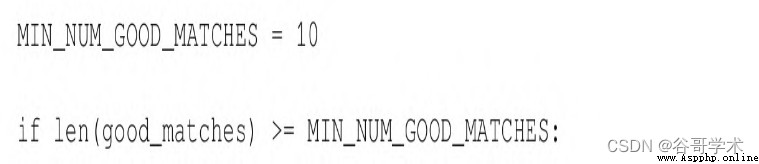
(2) Technically speaking , At least we can use 4 Matches to calculate homography . but
yes , If this 4 Any one of the matches is defective , Will destroy the accuracy of the results
sex . In practice, at least 10 Matches . For additional matches , Homography search algorithm
Method can discard some outliers , In order to produce knots that closely match most of the subset of matches
fruit . therefore , We continue to check whether there is at least 10 A good match :
(3) If this condition is met , Then find the two-dimensional coordinates of the matching key points ,
And put these coordinates into the two lists of floating-point coordinate pairs . A list contains query images
Coordinates of key points in , Another list contains the coordinates of the matching keys in the scene :

(4) Look for homography :
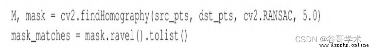
Please note that , We created mask_matches list , Will be used for final matching
system , In this way, only points that meet homography will draw match lines .
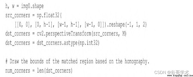
(5) At this stage , A perspective transformation must be performed , Take the rectangular corner of the query image
spot , And project it into the scene , In this way, the boundary can be drawn :
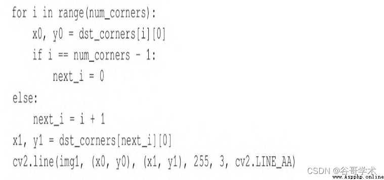
then , Continue to draw keys and display visualization , As in the previous example
sample .
6.10 Sample application : Tattoo evidence
We take a real life ( Or fantasy life ) To end this chapter .
Suppose you work in the forensic Department of a city , Need to identify a tattoo . You have the origin of Criminal Tattoo
Start picture ( It may be captured in the CCTV video ), But I don't know this person's
identity . But , You have a tattoo database , It is based on the name of the person to whom the tattoo belongs
lead .
We divide this task into two parts :
· Build the database by saving the image descriptor to a file .
· Load the database and scan the descriptor of the query image and the descriptor in the database
Matches .
In the next two sections , We will introduce these tasks .
6.10.1 Save image descriptor to file
The first thing we need to do is to save the image descriptor to an external file . such ,
We don't have to recreate the descriptor every time we scan two images to match .
For the purposes of this example , We scan an image folder , And create the corresponding descriptor
file , In this way, these contents can be used at any time in future search . To create a description
operator , We will use the method that has been used many times in this chapter : Load image 、 Create feature check
Tester 、 Detect features and calculate descriptors . To save the descriptor to a file , We will use
be known as save Of NumPy Convenient method of array , Dump the array data to Wen in an optimized way
In the piece .
stay Python Standard library ,pickle Module provides a more general serialization function ,
Support any Python object , not only NumPy Array . But ,NumPy Array sequence of
Digitization is a good choice for digital data .
We decompose the script into functions . The main function will be named
create_descriptors, It will traverse the files in a given folder . For each article
Pieces of ,create_descriptors Name the call create_descriptor Auxiliary function of ,
This function will calculate and save the descriptor of the given image file .
(1) First ,create_descriptors The implementation is as follows :
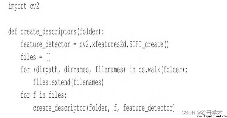
Be careful ,create_descriptors Created feature detector , Because we just need
To create a , Instead of creating each time a file is loaded . Auxiliary function
create_descriptor Receive the feature detector as a parameter .
(2) Now? , Let's look at the implementation of auxiliary functions :
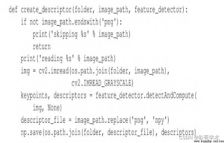
Be careful , We save the descriptor file in the same folder as the image . Besides ,
We assume that the image file has png Extension . To make the script more robust , It can be improved
Line modification , Make the script support additional image file extensions , Such as jpg. If the file has a
Unexpected extension , Just skip it , Because it may be a descriptor file ( From before
The script runs ) Or other non image files .
(3) We have completed the implementation of the function . To complete the script , We're going to call
create_descriptors, Use folder name as parameter :
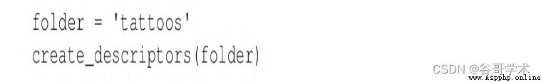
When running this script , It will generate NumPy The necessary descriptor of array file format
Pieces of , The file extension is npy. These files form the tattoo descriptor database , Search by name
lead .( Each file name is a personal name .) Next , We will write a separate
Script , In this way, you can query the database .
6.10.2 Scan matching
Now that the descriptor has been saved to a file , We only need to execute for each descriptor set
matching , To determine which set best matches the query image .
The following is the process to be implemented :
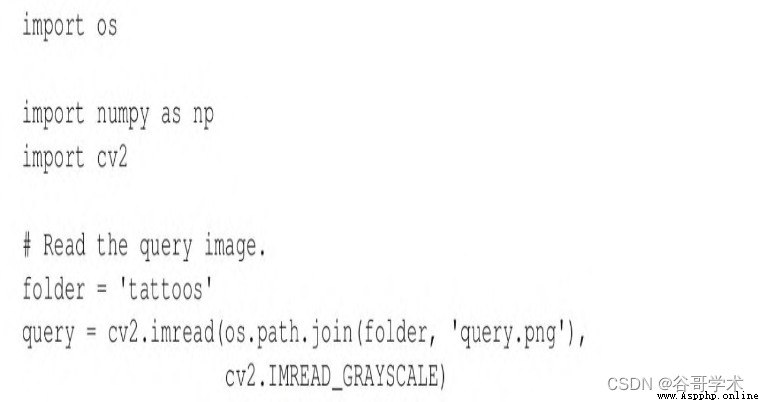
(1) Load query image (query.png).
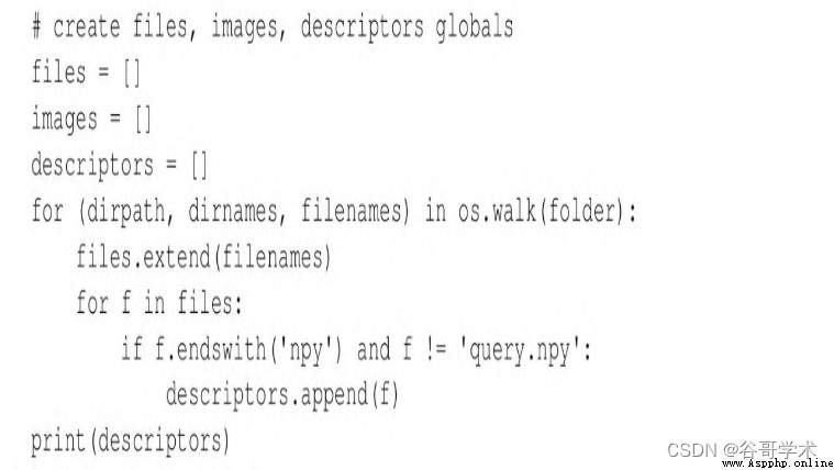
(2) Scan the folder containing the descriptor file . The name of the print descriptor file .
(3) Create for query image SIFT The descriptor .
(4) For each descriptor file , load SIFT The descriptor , And search based on FLANN
Matches for . Filter matches based on ratio checking . Print the name of this person and the number of matches
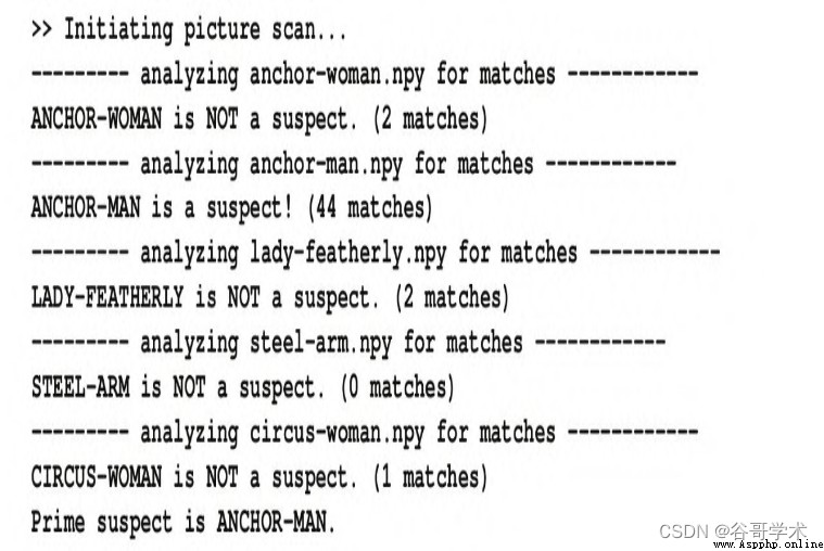
The amount . If the number of matches exceeds any threshold , Then print “ This person is a suspect ”.
( please remember , We are investigating a criminal activity .)
(5) Print the name of the main suspect ( The person with the most matches ).
Let's consider its implementation :
(1) First , Load the query image with the following code block :
(2) Compile and print a list of descriptor files :
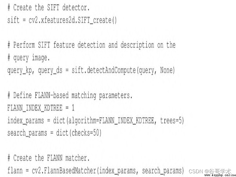
(3) Establish a typical cv2.SIFT and cv2.FlannBasedMatcher object , also
Generate the descriptor of the query image :
(4) Looking for suspects , Define the suspect as having at least 10 A good match with the query tattoo
The right person . The search process includes traversing descriptor files 、 Load descriptor 、 Execution is based on FLANN
The matching of , And filter matches based on ratio test . Print everyone ( Each descriptor
Pieces of ) Match results for :
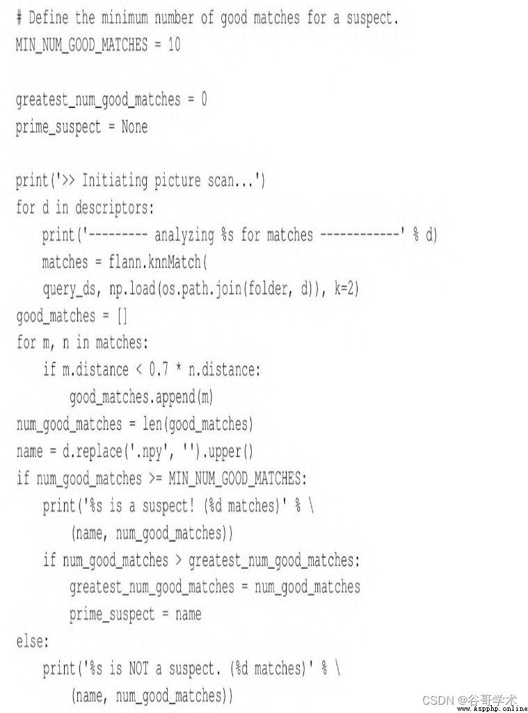
Be careful np.load Method usage , It will specify NPY File loading to NumPy
Array .
(5) Last , Print the name of the main suspect ( If the suspect is found ):
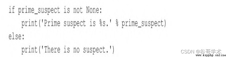
Run the above script , The output is as follows :
If you like , As you did in the previous section , You can also use graphics to represent matches
Coordination and homography .
6.11 Summary of this chapter
In this chapter , We introduced key point detection 、 Calculation of key descriptor 、 The descriptor
The matching of 、 Bad matching filtering , And finding homography between two groups of matching key points .
We talked about OpenCV Some algorithms that can be used to complete the above tasks in , And these algorithms
Applied to various images and use cases .
If the new knowledge about key points is combined with the knowledge of camera and perspective , I
We can track objects in three-dimensional space . This will be the second 9 Chapter theme . If you are very thirsty
Hope to enter the three-dimensional field , Then you can jump to the 9 Chapter to learn .
contrary , If you think the following content is useful for you to improve the relevant object detection 、 distinguish
And track the knowledge of two-dimensional solutions is helpful , Then you can continue to learn 7 Zhang He
8 Content of Chapter . It's best to know about two-dimensional and three-dimensional combination technology , In this way, you can choose to give
Determine how the application provides the correct output type and the appropriate calculation speed .