Through the foreshadowing of the previous chapters , We also have a little understanding of data processing . The main preference for follow-up is Pandas, It includes data structures and operational tools that make data cleaning and analysis faster and simpler .pandas Often used in parallel with other tools , Learned from the previous chapter numpy and scipy, Analysis Library statsmodels and scikit-learn, And data visualization Library matplotlib.pandas Is based on numpy The establishment of a , Especially for array based functions and not using for Cyclic data processing .
although pandas Used a lot of numpy Encoding style , But the biggest difference between the two is pandas A framework designed specifically to handle tables and mixed data . and numpy It is more suitable for processing uniform numerical array data .
In this chapter , I will introduce... Using the following conventions pandas:
In [1]: import pandas as pd
because Series and DataFrame Used a lot , Therefore, it is more convenient to introduce it into the local namespace :
In [2]: from pandas import Series, DataFrame
To use pandas, You first have to be familiar with its two main data structures :Series and DataFrame. These two basic numbers can solve most of the processing problems , So we need to understand their details .
Series Is an object similar to a one-dimensional array , It consists of a set of data ( Various numpy Data type of ) And a set of related data labels ( Indexes ) form .
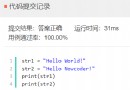
In [11]: obj = pd.Series([4, 7, -5, 3])
In [12]: obj
Out[12]:
0 4
1 7
2 -5
3 3
dtype: int64
Series On the left is the index , On the right is the data value . There is no special index setting for the data , So it is the default from 0 Starting index label . You can also pass Series Of values and index Property to access the contents of the array :
In [13]: obj.values
Out[13]: array([ 4, 7, -5, 3])
In [14]: obj.index # like range(4)
Out[14]: RangeIndex(start=0, stop=4, step=1)
Generally speaking , We hope Series Each data can be marked :
In [15]: obj2 = pd.Series([4, 7, -5, 3], index=['d', 'b', 'a', 'c'])
In [16]: obj2
Out[16]:
d 4
b 7
a -5
c 3
dtype: int64
In [17]: obj2.index
Out[17]: Index(['d', 'b', 'a', 'c'], dtype='object')
And ordinary NumPy Array comparison , You can select by index Series A single or set of values in :
In [18]: obj2['a']
Out[18]: -5
In [19]: obj2['d'] = 6
In [20]: obj2[['c', 'a', 'd']]
Out[20]:
c 3
a -5
d 6
dtype: int64
Of course, you can also learn from the previous chapter numpy Relevant knowledge of Series Do data operations :
In [21]: obj2[obj2 > 0]
Out[21]:
d 6
b 7
c 3
dtype: int64
In [22]: obj2 * 2
Out[22]:
d 12
b 14
a -10
c 6
dtype: int64
In [23]: np.exp(obj2)
Out[23]:
d 403.428793
b 1096.633158
a 0.006738
c 20.085537
dtype: float64
If the data is stored in a Python In the dictionary , You can also create... Directly from this dictionary Series:
In [26]: sdata = {'Ohio': 35000, 'Texas': 71000, 'Oregon': 16000, 'Utah': 5000}
In [27]: obj3 = pd.Series(sdata)
In [28]: obj3
Out[28]:
Ohio 35000
Oregon 16000
Texas 71000
Utah 5000
dtype: int64
If only one dictionary is passed in , Then the result Series The index in is the key of the original dictionary ( Arrange in order ). You can change the order by passing in the keys of the ordered dictionary :
In [29]: states = ['California', 'Ohio', 'Oregon', 'Texas']
In [30]: obj4 = pd.Series(sdata, index=states)
In [31]: obj4
Out[31]:
California NaN
Ohio 35000.0
Oregon 16000.0
Texas 71000.0
dtype: float64
In this case ,sdata and states Only when the index matches will it be stored in the newly generated object , because states Medium California Cannot find corresponding value , So for NaN. and Utah It's not in states in , So there is no .
such NaN stay pandas Is called loss value or NA value .pandas Have function isnull and notnull Detect whether the array contains loss values :
In [32]: pd.isnull(obj4)
Out[32]:
California True
Ohio False
Oregon False
Texas False
dtype: bool
In [33]: pd.notnull(obj4)
Out[33]:
California False
Ohio True
Oregon True
Texas True
dtype: bool
Of course, careful students may find Series A very important function is data alignment , The data can be arranged neatly , This is very helpful for our data analysis .Series The object itself and its index have a property name, This attribute and pandas Is closely related to other functions of :
In [38]: obj4.name = 'population'
In [39]: obj4.index.name = 'state'
In [40]: obj4
Out[40]:
state
California NaN
Ohio 35000.0
Oregon 16000.0
Texas 71000.0
Name: population, dtype: float64
meanwhile Series The index of can be modified in place by assignment :
In [41]: obj
Out[41]:
0 4
1 7
2 -5
3 3
dtype: int64
In [42]: obj.index = ['Bob', 'Steve', 'Jeff', 'Ryan']
In [43]: obj
Out[43]:
Bob 4
Steve 7
Jeff -5
Ryan 3
dtype: int64
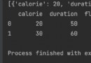
DataFrame Is a tabular data structure , It contains a set of sequences , Each column can identify different types of values .DataFrame Existing row index , There are also column indexes , It can be seen as Series A dictionary made up of .DataFrame The data in is stored in one or more two-dimensional blocks , Not a list , A collection of dictionaries or other one-dimensional arrays . About its internal implementation , This is beyond the scope of this chapter , So interested partners can consult and understand the details by themselves .
The first step in learning a new data structure is to learn how to construct it . There are many ways to construct DataFrame, The most common way is to use a list containing equal length or Numpy Array dictionary to form DataFrame:
data = {'state': ['Ohio', 'Ohio', 'Ohio', 'Nevada', 'Nevada', 'Nevada'],
'year': [2000, 2001, 2002, 2001, 2002, 2003],
'pop': [1.5, 1.7, 3.6, 2.4, 2.9, 3.2]}
frame = pd.DataFrame(data)
result DataFrame It will be indexed automatically ( Follow Series equally ):
In [24]:frame
Out[24]:
state year pop
0 Ohio 2000 1.5
1 Ohio 2001 1.7
2 Ohio 2002 3.6
3 Nevada 2001 2.4
4 Nevada 2002 2.9
5 Nevada 2003 3.2
If you're using Jupyter notebook,pandas DataFrame Object will be browser friendly HTML Table presentation . For a very large DataFrame,head Method will select the first five lines :
In [26]:frame.head()
Out[27]:
state year pop
0 Ohio 2000 1.5
1 Ohio 2001 1.7
2 Ohio 2002 3.6
3 Nevada 2001 2.4
4 Nevada 2002 2.9
If you want to customize the column order , You need to make a sequence :
In [27]:pd.DataFrame(data, columns=['year', 'state', 'pop'])
Out[28]:
year state pop
0 2000 Ohio 1.5
1 2001 Ohio 1.7
2 2002 Ohio 3.6
3 2001 Nevada 2.4
4 2002 Nevada 2.9
5 2003 Nevada 3.2
If the incoming column cannot be found in the data , Will produce missing values in the results :
In [28]:pd.DataFrame(data, columns=['year', 'state', 'pop', 'debt'],
....: index=['one', 'two', 'three', 'four',
....: 'five', 'six'])
Out[29]:
year state pop debt
one 2000 Ohio 1.5 NaN
two 2001 Ohio 1.7 NaN
three 2002 Ohio 3.6 NaN
four 2001 Nevada 2.4 NaN
five 2002 Nevada 2.9 NaN
six 2003 Nevada 3.2 NaN
By means of dictionary tags or attributes , Can be DataFrame Gets the column of as a Series:
In [36]:frame2['year']
Out[33]:
one 2000
two 2001
three 2002
four 2001
five 2002
six 2003
Name: year, dtype: int64
In [36]:frame2.state
Out[34]:
one Ohio
two Ohio
three Ohio
four Nevada
five Nevada
six Nevada
Name: state, dtype: object
Rows can also be obtained by location or name , For example, we use loc attribute :
In [36]:frame2.loc['three']
Out[36]:
year 2002
state Ohio
pop 3.6
debt NaN
Name: three, dtype: object
Columns can be modified by assignment . for example , We can give that empty "debt" Assign a scalar value or a set of values to a column :
In [37]: frame2['debt'] = 16
In [38]:frame2
Out[38]:
year state pop debt
one 2000 Ohio 1.5 16
two 2001 Ohio 1.7 16
three 2002 Ohio 3.6 16
four 2001 Nevada 2.4 16
five 2002 Nevada 2.9 16
six 2003 Nevada 3.2 16
In [39]: import numpy as np
In [40]: frame2['debt'] = np.arange(6.)
In [41]: frame2
Out[41]:
year state pop debt
one 2000 Ohio 1.5 0.0
two 2001 Ohio 1.7 1.0
three 2002 Ohio 3.6 2.0
four 2001 Nevada 2.4 3.0
five 2002 Nevada 2.9 4.0
six 2003 Nevada 3.2 5.0
When assigning a list or array to a column , Its length must follow DataFrame Match the length of . If the assignment is a Series, It will match exactly DataFrame The index of , All spaces will be filled with missing values :
In [42]: val = pd.Series([-1.2, -1.5, -1.7], index=['two', 'four', 'five'])
In [43]: frame2['debt'] = val
In [44]: frame2
Out[44]:
year state pop debt
one 2000 Ohio 1.5 NaN
two 2001 Ohio 1.7 -1.2
three 2002 Ohio 3.6 NaN
four 2001 Nevada 2.4 -1.5
five 2002 Nevada 2.9 -1.7
six 2003 Nevada 3.2 NaN
Assigning a value to a column that does not exist creates a new column . keyword del Used to delete columns . As del Example , I first add a new Boolean column ,state Is it 'Ohio':
In [45]: frame2['ear'] = frame2.state == 'Ohio'
In [46]: frame2
Out[46]:
year state pop debt ear
one 2000 Ohio 1.5 NaN True
two 2001 Ohio 1.7 -1.2 True
three 2002 Ohio 3.6 NaN True
four 2001 Nevada 2.4 -1.5 False
five 2002 Nevada 2.9 -1.7 False
six 2003 Nevada 3.2 NaN False
Be careful not to use frame2.eastern Create a new column .
del Method can be used to delete this column :
In [47]: del frame2['ear']
In [48]: frame2.columns
Out[48]: Index(['year', 'state', 'pop', 'debt'], dtype='object')
Be careful : The columns returned by indexing are just views of the corresponding data , Not a copy . therefore , For returned Series Any in place changes you make are reflected in the source DataFrame On . adopt Series Of copy Method to specify the replication column .
Another common form of data is nested dictionaries :
In [49]: pop = {'Nevada': {2001: 2.4, 2002: 2.9},
....: 'Ohio': {2000: 1.5, 2001: 1.7, 2002: 3.6}}
If the nested dictionary is passed to DataFrame,pandas It would be interpreted as : The key of the outer dictionary is the column , The inner key is used as the row index :
In [50]: frame3 = pd.DataFrame(pop)
In [51]: frame3
Out[52]:
Nevada Ohio
2000 NaN 1.5
2001 2.4 1.7
2002 2.9 3.6
You can also use something like NumPy Array method , Yes DataFrame To transpose ( Swap rows and columns ):
In [53]: frame3.T
Out[53]:
2000 2001 2002
Nevada NaN 2.4 2.9
Ohio 1.5 1.7 3.6
pandas The index object of is responsible for managing axis labels and other metadata ( For example, shaft name ). structure Series or DataFrame when , The tags of any array or other sequence used will be converted to Index:
In [76]: obj = pd.Series(range(3), index=['a', 'b', 'c'])
In [77]: index = obj.index
In [78]: index
Out[78]: Index(['a', 'b', 'c'], dtype='object')
In [79]: index[1:]
Out[79]: Index(['b', 'c'], dtype='object')
Index Object is immutable , Therefore, the user cannot modify it . Immutability can make Index Objects are safely shared among multiple data structures :
In [80]: labels = pd.Index(np.arange(3))
In [81]: labels
Out[81]: Int64Index([0, 1, 2], dtype='int64')
In [82]: obj2 = pd.Series([1.5, -2.5, 0], index=labels)
In [83]: obj2
Out[83]:
0 1.5
1 -2.5
2 0.0
dtype: float64
In [84]: obj2.index is labels
Out[84]: True
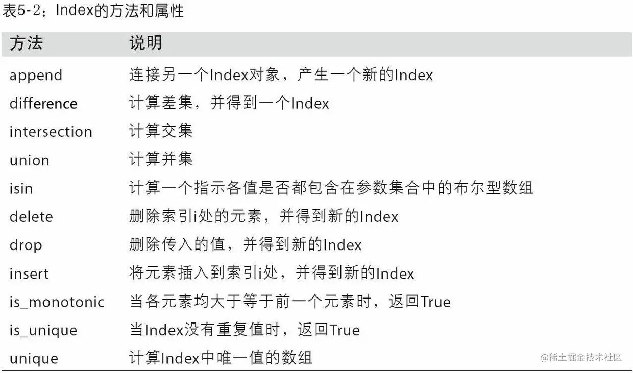
Here's the chart 5-2 Lists common methods and properties for indexing
The basic concepts are introduced , Next, we need to solve the basic means of data operation , This article is not an exhaustive list of pandas library , So just show some common functions , If you want to learn more , You can read the relevant documents carefully for further study .
reindex yes pandas An important method of object , This method is used to create a new object that matches the new index :
In [91]: obj = pd.Series([4.5, 7.2, -5.3, 3.6], index=['d', 'b', 'a', 'c'])
In [92]: obj
Out[92]:
d 4.5
b 7.2
a -5.3
c 3.6
dtype: float64
Use this Series Of reindex Will be rearranged according to the new index . If an index value does not currently exist , We introduce missing values :
In [93]: obj2 = obj.reindex(['a', 'b', 'c', 'd', 'e'])
In [94]: obj2
Out[94]:
a -5.3
b 7.2
c 3.6
d 4.5
e NaN
dtype: float64
For data with sequential structure , For example, incremental function , Interpolation and filling are required when rebuilding the index .method Method allows us to insert , for example ffill Method , Will be inserted before the value :
In [95]: obj3 = pd.Series(['blue', 'purple', 'yellow'], index=[0, 2, 4])
In [96]: obj3
Out[96]:
0 blue
2 purple
4 yellow
dtype: object
In [97]: obj3.reindex(range(6), method='ffill')
Out[97]:
0 blue
1 blue
2 purple
3 purple
4 yellow
5 yellow
dtype: object
stay DataFrame in ,reindex You can still change the index values of rows and columns . Just pass a sequence , The result will be reset :
In [98]: frame = pd.DataFrame(np.arange(9).reshape((3, 3)),
....: index=['a', 'c', 'd'],
....: columns=['Ohio', 'Texas', 'California'])
In [99]: frame
Out[99]:
Ohio Texas California
a 0 1 2
c 3 4 5
d 6 7 8
In [100]: frame2 = frame.reindex(['a', 'b', 'c', 'd'])
In [101]: frame2
Out[101]:
Ohio Texas California
a 0.0 1.0 2.0
b NaN NaN NaN
c 3.0 4.0 5.0
d 6.0 7.0 8.0
Columns can be columns Keyword re index :
In [102]: states = ['Texas', 'Utah', 'California']
In [103]: frame.reindex(columns=states)
Out[103]:
Texas Utah California
a 1 NaN 2
c 4 NaN 5
d 7 NaN 8
If you already have an indexed array or a list without entries , It is easy to delete one or more entries axially , But this requires some data manipulation and set logic ,drop Method returns a new object with an indicated value or an axially deleted value :
In [105]: obj = pd.Series(np.arange(5.), index=['a', 'b', 'c', 'd', 'e'])
In [106]: obj
Out[106]:
a 0.0
b 1.0
c 2.0
d 3.0
e 4.0
dtype: float64
In [107]: new_obj = obj.drop('c')
In [108]: new_obj
Out[108]:
a 0.0
b 1.0
d 3.0
e 4.0
dtype: float64
In [109]: obj.drop(['d', 'c'])
Out[109]:
a 0.0
b 1.0
e 4.0
dtype: float64
stay DataFrame in , There are similar attribute methods , I'm not going to show you , You can try it yourself . But use it with care drop Function inplace attribute , Careful use inplace, It will destroy all deleted data .‘
Series The index works in a way similar to Numpy, It's just Series There are richer index types :
In [117]: obj = pd.Series(np.arange(4.), index=['a', 'b', 'c', 'd'])
In [118]: obj
Out[118]:
a 0.0
b 1.0
c 2.0
d 3.0
dtype: float64
In [119]: obj['b']
Out[119]: 1.0
In [120]: obj[1]
Out[120]: 1.0
In [121]: obj[2:4]
Out[121]:
c 2.0
d 3.0
dtype: float64
In [122]: obj[['b', 'a', 'd']]
Out[122]:
b 1.0
a 0.0
d 3.0
dtype: float64
In [123]: obj[[1, 3]]
Out[123]:
b 1.0
d 3.0
dtype: float64
In [124]: obj[obj < 2]
Out[124]:
a 0.0
b 1.0
dtype: float64
DataFrame The method of operation is similar to Series. It can also be selected through the above methods . This makes DataFrame Grammar and NumPy The syntax of a two-dimensional array is very similar to .
about DataFrame The line of label ,pandas Introduced loc and iloc, They allow the user to communicate with the user through a process similar to numpy The way of marking , Use shaft labels (loc) Or integer label (iloc), from DataFrame Select a subset of rows and columns . The following is a preliminary example , Let's select one row or more columns through the tag :
In [137]: data.loc['Colorado', ['two', 'three']]
Out[137]:
two 5
three 6
Name: Colorado, dtype: int64
And then use iloc And integer , Numbers represent rows and columns :
In [138]: data.iloc[2, [3, 0, 1]]
Out[138]:
four 11
one 8
two 9
Name: Utah, dtype: int64
In [139]: data.iloc[2]
Out[139]:
one 8
two 9
three 10
four 11
Name: Utah, dtype: int64
In [140]: data.iloc[[1, 2], [3, 0, 1]]
Out[140]:
four one two
Colorado 7 0 5
Utah 11 8 9
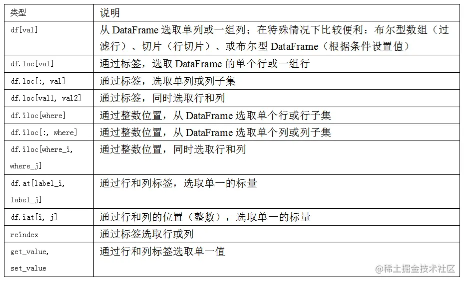
These two indexing functions are also applicable to slices of one label or multiple labels . therefore , stay pandas in , There are several ways to select and recombine data . about DataFrame, chart 5-1 It is summarized . You'll see that in the back , There are more ways to index hierarchically .
Due to too much content, there is one article here !!