Catalog
The first 4 Chapter Fundamentals of machine learning
4.1 Four branches of machine learning
4.1.1 Supervised learning
4.1.2 Unsupervised learning
4.1.3 Self supervised learning
4.1.4 Reinforcement learning
4.2 Evaluating machine learning models
4.2.1 Training set 、 Validation set and test set
4.2.2 Considerations for evaluating models
4.3 Data preprocessing 、 Feature Engineering and feature learning
4.3.1 Data preprocessing of neural network
4.3.2 Feature Engineering
4.4 Over fitting and under fitting
4.4.1 Reduce the network size
4.4.2 Add weight regularization
4.4.3 add to dropout Regularization
4.5 General workflow of machine learning
4.5.1 Define the problem , Collecting data sets
4.5.2 Choose a measure of success
4.5.3 Determine the evaluation method
4.5.4 Prepare the data
4.5.5 Develop better models than benchmarks
4.5.6 Expand the scale of the model : Developed fitted models
4.5.7 Model regularization and adjustment of hyperparameters
Summary of this chapter
Supervised learning is currently the most common type of machine learning , Given a set of samples ( Usually marked manually ), It can learn to map input data to known targets , In recent years, the widely concerned deep learning applications almost all belong to supervised learning , For example, optical character recognition 、 speech recognition 、 Image classification and language translation .
Supervised learning mainly includes classification and regression , But there are more exotic variants , It mainly includes the following :
1. Sequence generation . Given an image , Predict the text describing the image .
2. Syntax tree prediction . Give a sentence , Predict the syntax tree generated by its decomposition .
3. object detection . Given an image , Draw a bounding box around a specific target in the figure , This problem can also be expressed as a classification problem ( Given multiple candidate bounding boxes , Classify the targets in each box ) Or the joint problem of classification and regression ( Using vector regression to predict the coordinates of the bounding box ).
4. Image segmentation . Given an image , Draw a pixel level mask on a specific object .
Unsupervised learning refers to finding interesting transformations of input data without goals , Its purpose is data visualization 、 data compression 、 Data denoising or better understanding of the correlation in the data . Unsupervised learning is a necessary skill for data analysis , Before solving the problem of supervised learning , To better understand the dataset , It is usually a necessary step . Dimension reduction and clustering are well-known unsupervised learning methods .
Self supervised learning is a special case of supervised learning , It's different , It's worth falling into a separate category . Self supervised learning is supervised learning without manual labeling , You can think of it as supervised learning without human participation . The label still exists ( There is always something to supervise the learning process ), But they are generated from input data , Usually generated using heuristic algorithms . Self encoder is a famous example of self supervised learning , The goal of its generation is unmodified input . Supervised learning 、 The difference between self supervised learning and unsupervised learning is sometimes vague , These three categories are more like a continuum without clear boundaries , Self supervised learning can be reinterpreted as supervised learning or unsupervised learning , It depends on whether you focus on the learning mechanism or the application scenario .
In reinforcement learning , An agent receives information about its environment , And learn to choose actions that maximize their rewards .
Glossary of classification and regression :
Sample or input : Data points entering the model .
Prediction or output : The results from the model .
The goal is : True value . For external data sources , Ideally , The model should be able to predict the target .
Category : A set of labels to choose from in a classification problem .
label : Specific examples of category labeling in classification problems .
True value or annotation : All targets of the dataset , Usually collected manually .
Two classification : A classification task , Each input sample should be divided into two mutually exclusive categories .
Many classification : A classification task , Each input sample should be divided into more than two categories , Such as sorting handwritten Numbers .
Multi label classification : A classification task , Each input sample can be assigned multiple labels .
Scalar regression : The goal is the task of continuous scalar values .
Vector regression : The goal is a set of tasks with continuous values .
Small batch or batch : A small number of samples processed by the model at the same time ( The number of samples is usually 8~128).
As the training goes on , The performance of the model on the training data is always improving , But performance on unprecedented data is no longer changing or starting to decline .
The goal of machine learning is to get models that can be generalized , That is, a model that performs well on unprecedented data , Over fitting is the core difficulty . You can only control what you can observe , Therefore, it is very important to measure the generalization ability of the model reliably .
The focus of the evaluation model is to divide the data into three sets : Training set 、 Validation set and test set . Training models on training data , Evaluate the model on validation data . Once the best parameters are found , The last test on the test data .
If the model configuration is adjusted based on the performance of the model on the verification set , It will soon cause the model to over fit on the validation set , Even if you don't train the model directly on the validation set .
The key to this phenomenon is information leakage , Each time, the model superparameters are adjusted based on the performance of the model on the verification set , There will be some information about the validation data leaked into the model . If the parameter is adjusted only once for each time , So little information is leaked , The validation set can still reliably evaluate the model . But if you repeat this process many times ( Run an experiment , Evaluate... On the validation set , Then modify the model accordingly ), Then more and more information about the validation set will be leaked into the model .
Last , The model you get performs very well on the validation set ( Man made ), Because that's the purpose of your optimization . What you care about is the performance of the model on new data , Instead of performance on validation data , So you need to use a completely different 、 An unprecedented data set to evaluate the model , It's the test set . Your model must not read any information about the test set , Not even indirect reading . If the model is adjusted based on the performance of the test set , Then the measurement of generalization ability is inaccurate .
Three classic evaluation methods : Simple verification 、K Fold validation , And duplication with scrambled data K Fold validation .
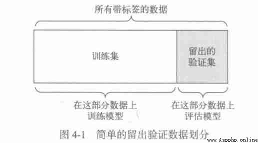
1. Simple verification
Set aside a certain proportion of data as a test set , Train the model on the remaining data , Then evaluate the model on the test set , As mentioned earlier , To prevent information leakage , You can't adjust the model based on the test set , So you should also keep a validation set .
Allow for verification :
num_validation_samples = 10000
np.random.shuffle(data)
data = data[num_validation_samples:]
training_data = data[:]
model = get_model()
model.train(training_data)
validation_score = model.evaluate(validataion_data)
model = get_model()
model.train(np.concatenate([training_data, validation_data]))
test_score = model.evaluate(test_data)
This is the simplest way to evaluate , But there is a drawback : If there is little data available , Then maybe the validation set and test set contain too few samples , Therefore, it is impossible to represent the data statistically .
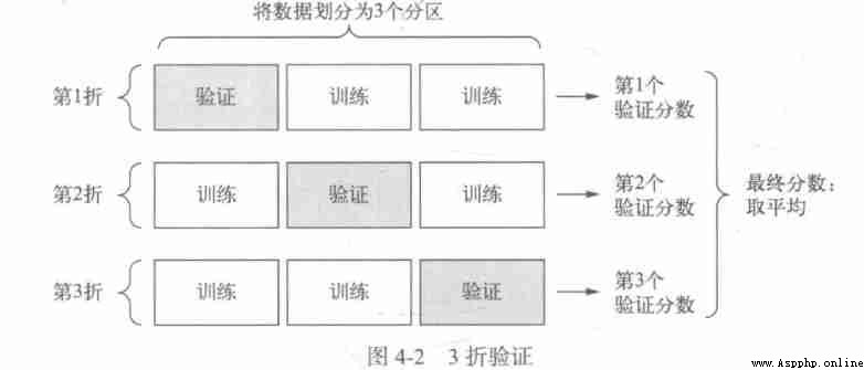
2.K Fold validation
K It divides the data into the same size K Zones , For each partition i, In the remaining K-1 Training model on two zones , Then partition i Upper evaluation model . The final score is equal to K The average of the scores . For different training sets - Test set partitioning , If the performance of the model changes greatly , So this method is very useful . As with validation , This method also requires independent validation sets for model correction .
K Crossover verification :
import numpy as np
k = 4
num_validation_samples = len(data) // k
np.random.shuffle(data)
validation_scores = []
for fold in range(k):
validation_data = data[num_validation_samples * fold : num_validation_samples * (fold + 1)]
training_data = data[:num_validation_samples * fold] + data[num_validation_samples * (fold + 1):]
model = get_model()
model.train(training_data)
validation_score = model.evaluate(validation_data)
validation_scores.append(validation_score)
validation_score = np.average(validation_scores)
model = get_model()
model.train(data)
test_score = model.evaluate(test_data)
3. Duplication with scrambled data K Fold validation
If there is relatively little data available , And you need to evaluate the model as accurately as possible , Then you can choose repetition with scrambled data K Fold validation . This method needs training and evaluation PxK A model (P It's the number of repetitions ), It's expensive to calculate .
1. Data representativeness . You want the training set and the test set to represent the current data , Before dividing the data into training sets and test sets , Usually the data should be randomly scrambled .
2. Time Arrow . If you want to predict the future from the past , So before dividing the data, you should not randomly disrupt the data , Because doing so will cause time leakage : Your model will be effectively trained in future data . under these circumstances , You should always make sure that all data in the test set is later than the training set .
3. data redundancy . If some data points in the data appear twice , Then disrupting the data and dividing it into training set verification sets leads to data redundancy between training set verification sets . In terms of effect , You are evaluating the model on some training data , Make sure there is no intersection between the training set and the verification set .
The purpose of data preprocessing is to make the original data more suitable for neural network processing , Including vectorization 、 Standardization 、 Deal with missing values and feature extraction .
1. To quantify
All inputs and targets of neural networks must be floating point tensors ( In a particular case, it can be an integer tensor ). No matter what data is processed ( voice 、 Image or text ), Must first be transformed into a tensor , This step is called data vectorization .
2. Value standardization
Generally speaking , The data with relatively large value ( For example, multiple integers , Much larger than the initial value of the network weight ) Or heterogeneous data input into neural network is unsafe , Doing so may result in large gradient updates , Thus, the network cannot converge . In order to make online learning easier , The input data should have the following characteristics .
(1) The value is small : Most values should be in 0~1 Within the scope of .
(2) Homogeneity : The values of all features should be in roughly the same range .
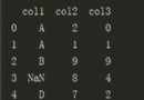
3. Handling missing values
Sometimes there may be missing values in your data , Generally speaking , For neural networks , Set the missing value to 0 Is safe , as long as 0 Not a meaningful value . The network can learn from data 0 Means missing data , And ignore this value .
If there may be missing values in the test data , The network is trained on data without missing values , Then the network cannot learn to ignore missing values . under these circumstances , You should artificially generate some training samples with missing items : Copy some training samples several times , Then delete some features that may be missing from the test data .
Feature engineering refers to the process of inputting data into a model , Use your own data and machine learning algorithms ( This is neural networks ) Hard coded transformation of data with knowledge of ( It's not the model ), To improve the effect of the model . Most of the time , A machine learning model cannot learn from completely arbitrary data , The data presented to the model should be easy for the model to learn .
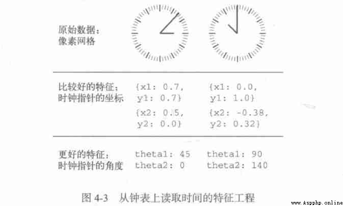
The essence of Feature Engineering : Express the problem in a simpler way , It makes the problem easier , It usually requires a deep understanding of the problem .
Before the advent of deep learning , Feature engineering used to be very important , Because the classical shallow algorithm does not have enough hypothesis space to learn useful representations by itself , The way the data is presented to the algorithm is crucial to solving the problem .
Fortunately, , For modern deep learning , Most feature engineering is unnecessary , Because neural network can automatically extract useful features from the original data , But this does not mean that only deep neural networks , There is no need to worry about Feature Engineering , This is because good features can still enable you to solve problems more gracefully with less resources , It also allows you to solve problems with less data .
Over fitting exists in all machine learning problems , Learning how to deal with over fitting is crucial to mastering machine learning .
The fundamental problem of machine learning is the opposition between optimization and generalization . Optimization refers to adjusting the model to get the best performance on the training data ( Learning in machine learning ), Generalization refers to the performance of the trained model on unprecedented data . The goal of machine learning is, of course, to get good generalization , But you can't control generalization , The model can only be adjusted based on training data .
At the beginning of training , Optimization and generalization are related : The smaller the loss in training data , The smaller the loss on the test data , At this time, the model is under fitting , There is still room for improvement , The network has not yet modeled all the relevant patterns in the training data . But after a certain number of iterations on the training data , Generalization no longer improves , The verification index is unchanged at first , And then it started to get worse , That is, the model begins to over fit . At this point, the model begins to learn patterns that are only related to training data , But this pattern is wrong or irrelevant for new data .
To prevent models from learning wrong or irrelevant patterns from training data , The best solution is to get more training data . The more training data the model has , The generalization ability is naturally better . If you can't get more data , The suboptimal solution is to adjust the amount of information allowed to be stored in the model , Or constrain the information that the model allows to store . If a network can only remember a few patterns , So the optimization process forces the model to focus on the most important patterns , This is more likely to get good generalization .
This method of reducing over fitting is called regularization .
The simplest way to prevent over fitting is to reduce the size of the model , That is to reduce the number of learnable parameters in the model ( This is determined by the number of layers and the number of units per layer ). In deep learning , The number of learnable parameters in a model is usually called the capacity of the model . intuitively , Models with more parameters have more memory capacity , Therefore, we can easily learn the perfect dictionary mapping between the training sample and the target , This kind of mapping doesn't have any generalization ability . Deep learning models are good at fitting training data , But the real challenge is to generalize , Instead of fitting .
On the contrary , If the memory resources of the network are limited , You can't easily learn this mapping . therefore , To minimize the loss , The network must learn the compressed representation of the target with strong prediction ability , This is the data representation that we are interested in . At the same time, the model you use should have enough parameters , To prevent under fitting , That is, the model should avoid the lack of memory resources . Find a trade-off between over capacity and under capacity .
But no magic formula can determine the best number of layers or the best size of each layer , You have to evaluate a range of different network architectures ( Of course, on the validation set , Not on the test set ), In order to find the best model size for the data . To find the right model size , The general workflow is to select relatively few layers and parameters at the beginning , Then gradually increase the size of the layer or add a new layer , Until this increase has little impact on the verification loss .
Original model :
from keras import models
from keras import layers
model = models.Sequential()
model.add(layers.Dense(16, activation='relu', input_shape=(10000,)))
model.add(layers.Dense(16, activation='relu'))
model.add(layers.Dense(1, activation='sigmoid'))
Smaller models :
model = model.Sequential()
model.add(layers.Dense(4, activation='relu', input_shape=(10000,)))
model.add(layers.Dense(4, activaiton='relu'))
model.add(layers.Dense(1, activaiton='sigmoid'))
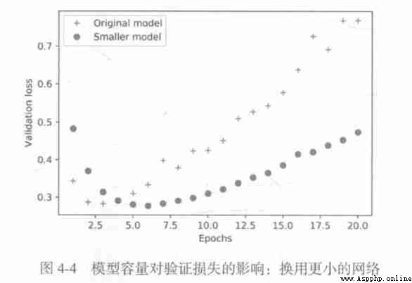
Pictured , Smaller networks start over fitting later than reference networks , And after the start of fitting , It's getting worse and slower .
Larger capacity models :
model = model.Sequential()
model.add(layers.Dense(512, activation='relu', input_shape=(10000,)))
model.add(layers.Dense(512, activation='relu'))
model.add(layers.Dense(1, activation='sigmoid'))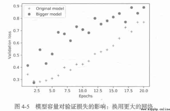
The larger networks start to over fit after only one round , Over fitting is more serious , Its verification losses are also more volatile .
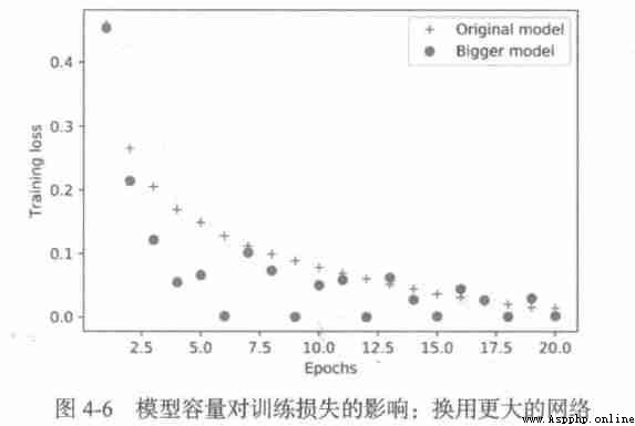
The training comfort of the larger network will soon be close to zero , The larger the capacity of the network , It fits the training data ( That is to say, we get a small training loss ) And the faster , But it's also easier to over fit ( There is a big difference between training loss and verification loss ) .
Occam's razor principle : If there are two explanations for a thing , Then the most likely correct explanation is the simplest one , Let's assume that the less . This principle also applies to the models learned by neural networks : Given some training data and a network architecture , A lot of group weight values ( A lot of models ) Can explain the data , Simple models are less likely to over fit than complex models .
The simple model here refers to the model with smaller entropy of parameter value distribution ( Or models with fewer parameters ), therefore , A common way to reduce over fitting is to force the weight of the model to be smaller , So as to limit the complexity of the model , This makes the distribution of weight values more regular . This method is called weight regularization , The implementation method is to add the cost related to the larger weight value to the network loss function . There are two forms of this cost :
1.L1 Regularization : The added cost is directly proportional to the absolute value of the weighting coefficient ;
2.L2 Regularization : The added cost is proportional to the square of the weighting coefficient . Neural network L2 Regularization is also called weight decay .
stay Keras in , The method of adding weight regularization is to pass the instance of weight regularization item to the layer as a keyword parameter .
Add to model L2 Weight regularization :
from keras import regularizers
model = model.Sequential()
model.add(layers.Dense(16, kernel_regularizer=regularizers.l2(0.001), activation='relu', input_shape=(10000,)))
model.add(layers.Dense(16, kernel_regularizer=regularizers.l2(0.001), activation='relu'))
model.add(layers.Dense(1, activation='sigmoid'))
Because this penalty item is only added during training , Therefore, the training loss of this network will be much greater than the test loss .
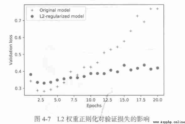
Even if the two models have the same number of parameters , have L2 The regularized model is more difficult to over fit than the reference model .
Keras Different weight regularization terms in :
from keras import regularizers
regularizers.l1(0.001)
regularizers.l1_l2(l1=0.001, l2=0.001)dropout It is one of the most effective and commonly used regularization methods for neural networks . Use... For a layer dropout, In the process of training, some output features of this layer are discarded randomly ( Set to 0).dropout The ratio is set to 0 The proportion of the characteristics of , Usually in 0.2~0.5 Within the scope of , No units are discarded during testing , And the output value of this layer needs to press dropout The ratio shrinks , Because more units are activated than during training , There needs to be a balance .
When testing :
layer_output *= np.random.randint(0, high=2, size=layer_output.shape)
layer_output *= 0.5
During training :
layer_output *= np.random.randint(0, high=2, size=layer_output.shape)
layer_output /= 0.5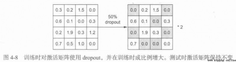
stay Keras in , You can go through Dropout Layer into the network dropout,dropout Will be applied to the output of the previous layer .
towards IMDB Add... To the network dropout:
model = models.Sequential()
model.add(layers.Dense(16, activation='relu', input_shape=(10000,)))
model.add(layers.Dropout(0.5))
model.add(layers.Dense(16, activation='relu'))
model.add(layers.Dropout(0.5))
model.add(layers.Dense(1, activation='sigmoid'))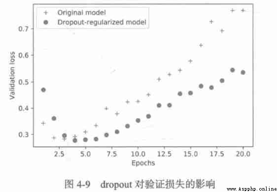
To sum up , Common methods to prevent neural network over fitting include :
1. Get more training data ;
2. Reduce network capacity ;
3. Add weight regularization ;
4. add to dropout.
First , You have to define the problem you face .
1. What is your input data ? What do you want to predict ? Only with available training data , You can learn to predict something .
2. What kind of problems are you facing ? It's a dichotomy problem 、 Multiple classification problem 、 Scalar regression problem 、 Vector regression problem , Or more classification 、 Multi label problem ? Or something else , For example, clustering 、 Generative or reinforcement learning ? Identifying the type of problem helps you choose the model architecture 、 Loss function, etc .
Only clear input 、 Output and data used , You can go to the next stage , Pay attention to the assumptions you make at this stage .
1. Suppose that the output can be predicted according to the input .
2. Suppose the available data contains enough information , Enough to learn the relationship between input and output .
Before developing a working model , These are just assumptions , Wait to verify the authenticity , Not all problems can be solved . You have collected the input X And the target Y Many examples of , It doesn't mean that X Contain enough information to predict Y.
There are some unsolvable problems you should know , That is the nonstationary problem . The object you want to model changes over time , under these circumstances , The correct approach is to constantly use the latest data to retrain the model , Or collect data on a stable time scale .
Machine learning can only be used to remember the patterns existing in the training data , You can only recognize what you've seen , Training machine learning on past data to predict the future , There's a hypothesis here , The law of the future is the same as that of the past , But this is often not the case .
To control one thing , You need to be able to observe it , To succeed , We must give a definition of success . The measure of success will guide you to choose the loss function , That is, what the model should optimize , It should be directly aligned with your goals .
For the balanced classification problem ( Each category may be the same ), Accuracy and the area under the receiver operating characteristic curve are commonly used indicators ; For the problem of category imbalance , You can use accuracy and recall ; For scheduling problems or multi label classification , You can use the average accuracy mean .
Once the goal is clear , You have to decide how to measure current progress .
1. Set aside validation sets .
2.K Crossover verification .
3. Repetitive K Fold validation .
Once you know what to train 、 What to optimize and how to evaluate , Then you're almost ready for the training model . But first you should format the data , So that it can be input into the machine learning model .
1. The data should be formatted as tensors .
2. The values of these tensors should usually be scaled to smaller values , For example [-1,1] Interval or [0,1] Section .
3. If different features have different value ranges ( Heterogeneous data ), Then data standardization should be done .
4. For small data problems, you may need to do feature Engineering .
After preparing the tensor of input data and target data , You can start training the model .
The goal of this stage is to obtain statistical efficacy , That is to develop a small model , It can beat a purely random benchmark .
Be careful , Statistical power is not always available , If you try a variety of reasonable architectures and still can't beat the random benchmark , Then the reason may be that the answer to the question is not in the input data , Remember the two assumptions you make :
1. Suppose that the output can be predicted according to the input .
2. Suppose the available data contains enough information , Enough to learn the relationship between input and output .
These assumptions are likely to be wrong , In that case, you need to start all over again .
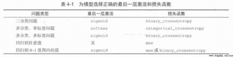
If all goes well , Three key parameters need to be selected to build the first working model :
1. Activation of the last layer . It effectively limits the network output .
2. Loss function . It should match the type of problem you want to solve
3. Optimize configuration .
On the choice of loss function , We need to pay attention to , Direct optimization of indicators to measure the success of a problem is not always feasible . Sometimes it is difficult to convert the index into a loss function , The loss function can be calculated when there is only a small batch of data ( Ideally , When there is only one data point , The loss function should also be computable ), And it must be differentiable ( Otherwise, the network cannot be trained by back propagation ).
Once you get a model with statistical power , The problem becomes : Is the model strong enough ? Does it have enough layers and parameters to model the problem ? The ubiquitous opposition in machine learning is the opposition between optimization and generalization , The ideal model is just on the boundary between under fitting and over fitting , On the line between insufficient capacity and excessive capacity . To find this line , You have to go through it .
To figure out how big a model you need , We have to develop an over fitting model .
1. Add more layers .
2. Make every layer bigger .
3. Train more rounds .
Always monitor training losses and validation losses , And the training value and verification value of the index you care about . If you find that the performance of the model on validation data begins to degrade , So there's overfitting .
This is the most time-consuming step : You're going to constantly adjust the model 、 Training 、 Evaluate... On validation data ( This is not the test data )、 Adjust the model again , And then repeat the process , Until the model reaches its best performance .
1. add to dropout.
2. Try different architectures : Increase or decrease the number of layers .
3. add to L1 and / or L2 Regularization .
4. Try different super parameters ( For example, the number of units in each layer or the learning rate of the optimizer ), To find the best configuration .
5. Do feature engineering over and over again : Add new features or delete features without information .
Each time you use feedback from the validation process to adjust the model , Will leak information about the validation process into the model . If you just repeat it a few times , So it doesn't matter ; But if you iterate systematically many times , Eventually, the model will over fit the validation process ( Even if the model is not trained directly on the validation data ), This reduces the reliability of the verification process .
Once a satisfactory model configuration is developed , You can get all the available data ( Training data + Validation data ) Train the final production model , And then one final evaluation on the test set . If the performance on the test set is much worse than that on the validation set , Then this means that your verification process is unreliable , Or you over fit the validation data when you adjust the model parameters , under these circumstances , You may need to switch to a more reliable assessment method , Like repeated K Fold validation .
1. Define the problem and the data to be trained . Collect the data , Label the data if necessary .
2. Choose indicators to measure the success of the problem .
3. Determine the evaluation method .
4. Develop the first better model than the benchmark , That is, a model with statistical effect .
5. Developed fitted models .
6. Based on the performance of the model on the validation data, the model is regularized and the hyperparameters are adjusted .