List of articles

• 0. Basic concepts
• • Series
  • • （ One ） establish Series
    • （ Two ）Series Simple operation of
  • DataFrame
  • • （ One ） establish DataFrame
• 1. Data selection
• • 1.1 [[]]
  • 1.2 copy()
  • 1.3 Column operation
  • 1.4 Line operation
  • 1.5 That's ok - Column
  • 1.6 Data filtering
• 2. Load data
• • 2.1 Txt
  • 2.2 Csv
  • Excel
• 3. Sorting and merging
• • 3.1 Series Sort
  • 3.2 DataFrame Sort
  • 3.3 Rank
  • 3.4 merge（ Match merge by column ）
  • 3.5 concat（ Data splicing ）
• 4. Data summary
• • 4.1 Special values （info, describe）
  • 4.2 Grouping statistics
• 5. The time series
• • 5.1 Initialize time series
  • 5.2 Time index
  • 5.3 Resampling
• Reference material

0. Basic concepts

Pandas The data type of is a table , You can put Pandas It can be understood as a memory database .

import pandas as pd

Series： Column
DataFrame： surface

Series

（ One ） establish Series

1. Use list list establish Series
（1） The default list index is from 0 - n-1

# Use list List Initialization sequence , The index value defaults to 0-n
ser = pd.Series([' Zhang San ', ' Li Si ', ' Wang Wu '])
ser

0 Zhang San
1 Li Si
2 Wang Wu
dtype: object

（2） Can pass index Parameter specifies the index value

ser = pd.Series([' Zhang San ', ' Li Si ', ' Wang Wu '], index = list(range(1,4))) # index Specifies the index value 
ser

1 Zhang San
2 Li Si
3 Wang Wu
dtype: object

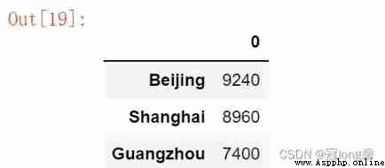
2. Using dictionaries dict establish Series
（1） The default index value is... Of the dictionary ’key’ value

data = {
'Beijing': 9240, 'Shanghai': 8960, 'Guangzhou': 7400}
ser3 = pd.Series(data)
ser3

Beijing 9240
Shanghai 8960
Guangzhou 7400
dtype: int64

（ Two ）Series Simple operation of

1. Modify element values
（1） Modify individual element values
Need to specify index , You can modify the element value of the specified index .
（2） Modify the element value of the whole column
Direct pair Series operation , The entire column of element values will be modified

ser2 = pd.Series([18, 19, 20], index = range(1,4))
ser2 + 1

1 19
2 20
3 21
dtype: int64

2. Type conversion

ser3.to_frame()

DataFrame

（ One ） establish DataFrame

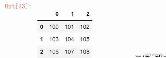
1. from numpy establish
numpy Initialize the created DataFrame The index of （index） And listing （columns） It's all by 0 - n-1 The numbers make up .

import numpy as np
data = np.arange(100, 109).reshape(3, -1)
df = pd.DataFrame(data)
df

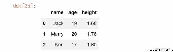
2. from dict establish
dict Initialize the created DataFrame The column with dict Of key Values remain the same

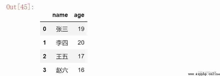
data = {

'name':['Jack', 'Marry', 'Ken'],
'age': [19, 20, 17],
'height': [1.68, 1.76, 1.80]
}
df = pd.DataFrame(data)
df

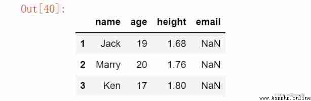
3. Index and column names
Can pass .columns Get column name ,.index Get index . You can specify indexes and column names at initialization or change them later

df1 = pd.DataFrame(data, columns=['name','age','height','email'], index = range(1,4))
df1

# To get the column name 
df.columns
# Index information 
df.index
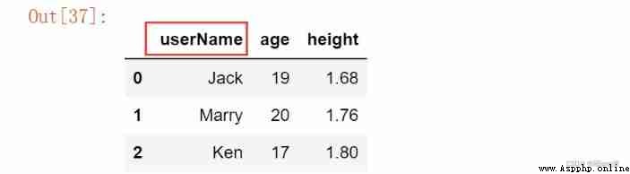
# Change column names 
df.columns = ['userName', 'age', 'height']
# Modify row index 
df.index = ['ABC'] # Assign values through strings 
df.index = range(df.shape[0])
df

Index([‘name’, ‘age’, ‘height’], dtype=‘object’)
RangeIndex(start=0, stop=3, step=1)

1. Data selection

1. Index： return DataFrame Index list of rows , Commonly used for index slicing
2. Columns： return DataFrame Column index , Commonly used for indexing and slicing
3. loc： return DataFrame Specify the rows of the custom index
4. iloc： return DataFrame Specify rows that are really positional indexes
   Be careful ：loc[], columns[] Are all index vectors .
5. shape： return DataFrame Row number 、 A list of the number of columns
6. drop(index , axis = )： Delete specified index , Designated line （0） Column （1） The elements of
7. [], [[]]： Respectively by Series and DataFrame Form from DataFrame Read data from
8. iat[x, y]： Returns the specified row and column elements

1.1 [[]]

Need to take out DataFrame When a certain column , Get is Series Variable . Sometimes the columns that need to be taken out are DataFrame Format .

# Take out a column (Series Format )
df['name']
df.name
# DataFrame Format 
df[['name', 'age']]

0 Zhang San
1 Li Si
2 Wang Wu
3 Zhao Liu
Name: name, dtype: object

1.2 copy()

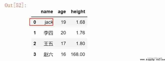
because DataFrame Characteristics of , The modification of an extracted column will affect the value of the main table . When the column data extracted from the column needs to be modified independently , May adopt copy() function .

names = df.name.copy()
names[0] = ' Zhang San '
names
df

0 Zhang San
1 Li Si
2 Wang Wu
3 Zhao Liu
Name: name, dtype: object

1.3 Column operation

Including the addition of columns 、 Delete 、 Change 、 check
1. Add column
Add a new column directly through the index value

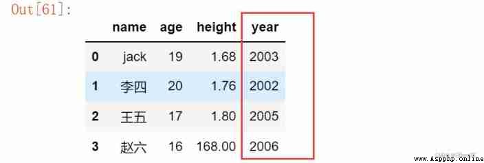
import datetime # Get the date of birth 
df['year'] = datetime.datetime.now().year - df.age
df

2. Delete the specified column
df.drop( Indexes ,axis = 1)：axis The default is 0, Said line .

df1 = df.drop('year', axis = 1) # The default is 0, When deleting a column, it needs to be specified as 1
df1

Be careful ：drop() Function does not change the calling object itself , To get the value, you need to save it with a new variable

3. Modify a column element
adopt [] or [[]] Get a column , Modify the specified element . This revision will affect DataFrame.

4. View a column of elements
Use “[]” or “[[ ]]” With Series or DataFrame Output a column or columns in the format of

1.4 Line operation

Including the addition of lines 、 Delete 、 Change 、 check
1. Add a row at the specified position
.loc[] The element that can return the specified index value row .DataFrame[] You can directly manipulate column elements , You need to add loc[] function

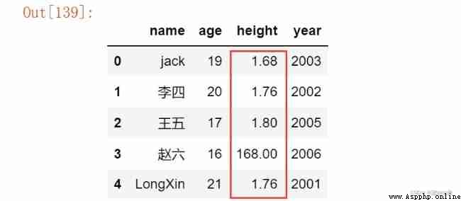
# Insert... In the last line 
df.loc[df.shape[0]] = {
'age':21,'name':'LongXin','height':1.76,'year':2001}
df

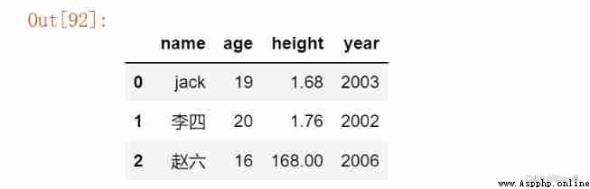
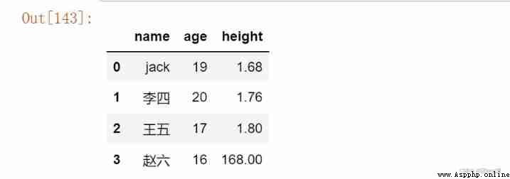
2. Delete specified row

1. adopt .drop() function , Delete the row of the specified index

df = df.drop(df.shape[0]-1, axis =0)
df = df.drop(2, axis =0)
df

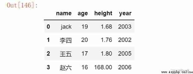
After deleting , Missing... In row index 2, Therefore, the row index needs to be updated again

2. adopt index function , Restore row index

df.index = range(df.shape[0])
df

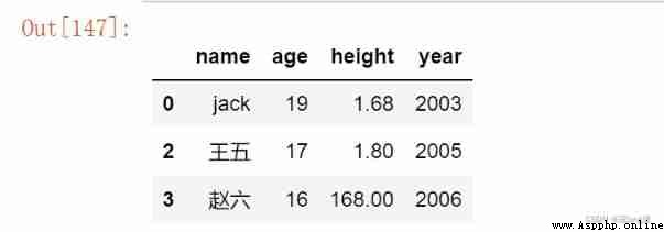
3. Find a line element

• loc[]： Search according to the customized index value , The row index must have the specified index value , Otherwise, an error will be reported .
• iloc[]： Find according to the index value of the physical location , There is not necessarily a specified index value in the row index

1.5 That's ok - Column

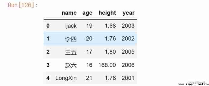
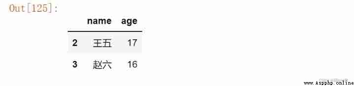
When we want to find the specified line 、 When specifying Columns , May adopt loc[] Combine row index and column index 、iat[] Direct index
for example , We want to get the countdown 2 That's ok ,'age’ and ’name’ Columns of data

df.loc[df.index[-2:], ['name', 'age']]
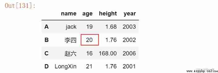
df

df1
df1.iat[1,1] = 66
df1


1.6 Data filtering

• Filter specified range data
• Filter the specified element data
• [ ], loc
• query(’’)
• isin

（1） Filter specified range data
have access to [], loc, query() Three methods are used to filter out the data in the specified range .
Method 1 ：[ [ Judgment statement ] ] nesting
Output all columns of all rows of the composite condition

df['height'] >= 1.65
df[df['height'] >= 1.65]

0 True
1 True
2 True
3 True
4 True
Name: height, dtype: bool

Method 2 ：loc( Judgment statement , Specified column )
stay [ [ ] ] On the basis of , Sure Output the specified column elements of all rows of the composite condition .

df.loc[(df['height'] >= 1.65)&(df['age']<=20),['name', 'age', 'height']]

Method 3 ：query(‘ character string ’)
By judging the string , Output qualified data . Effect and [ [ Judge ] ] identical .

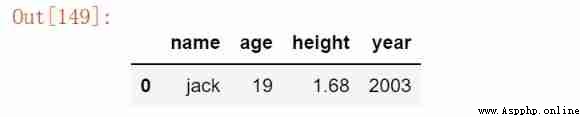
df.query('height >=1.65 and age <=20 or name == "jack" ')
age = 20
df.query('age < @age') # @ Variable 

Method four ：isin()
Determine whether the element is in the specified column , Then return the specified element

# isin() Determine whether an element exists 
df['age'].isin([18,19])
df[df['age'].isin([18,19])]

0 True
1 False
2 False
3 False
4 False
Name: age, dtype: bool

2. Load data

1. Text
2. CSV
3. Excel
4. Html
5. MySQL

2.1 Txt

adopt pd.read_table Function can read txt file , There are the following important parameters

• sep： The default is tab, Specify the separator
• header： Default first line column name , choice None May cancel
• names： Set column name manually , The default is 0-n

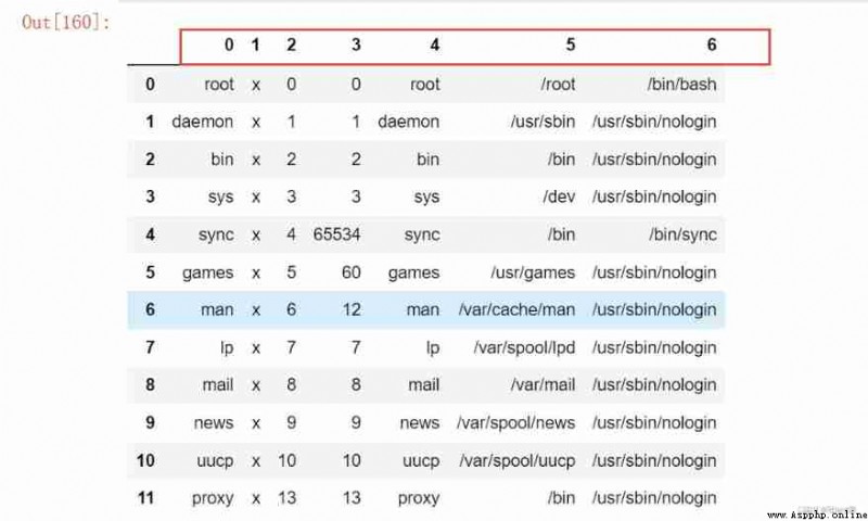
pd.read_table('D:\\Jupyter_notebook\\pandas_data\\03.txt', sep = ':', header =None )
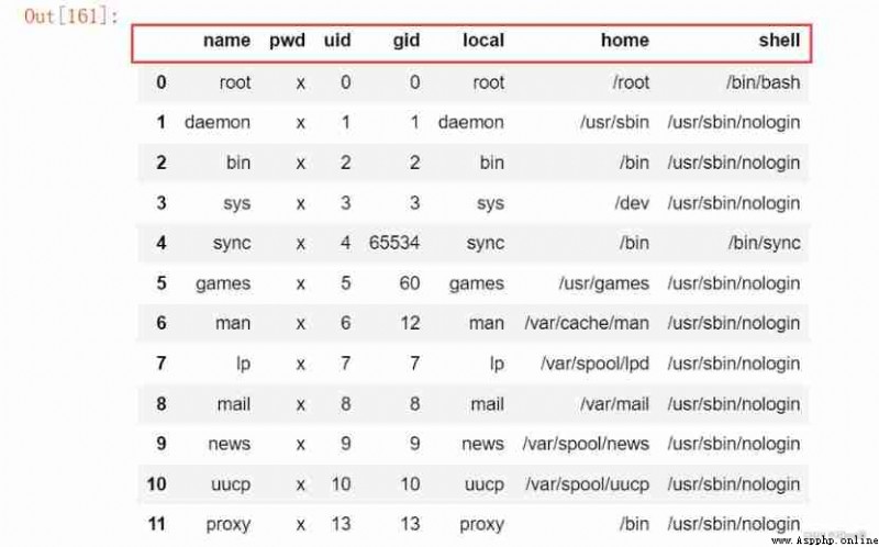
pd.read_table('D:\\Jupyter_notebook\\pandas_data\\03.txt', sep = ':', header =None, names = ['name', 'pwd', 'uid', 'gid', 'local', 'home', 'shell'] )

2.2 Csv

adopt pd.read_csv File read ,csv The file is , File with delimiter . The important parameters are as follows

• header： Default first line column name , choice None May cancel

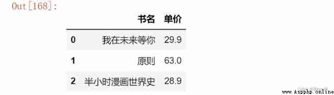
# csv Data from , Segmentation 
pd.read_csv('D:\\Jupyter_notebook\\pandas_data\\04.csv')

Excel

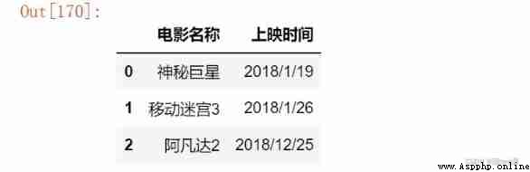
Need to introduce xlrd package , adopt pd.read_excel() Read excel file . The important parameters are as follows ：

• header： Default first line column name , choice None May cancel

# Excel
import xlrd
pd.read_excel('D:\\Jupyter_notebook\\pandas_data\\05.xlsx')

3. Sorting and merging

1. Sort
2. rank
3. merge
4. Concat

3.1 Series Sort

• sort_index(ascending = True)： Sort by serial number , The default is True That is, in ascending order
• sort_values(ascending = True)： Sort by value , The default is True That is, in ascending order

3.2 DataFrame Sort

• sort_index(axis = 0, ascending = True)： Sort by row or column ordinal (0 or 1), The default is 1 and True That is, in ascending order of line serial number
• sort_values(by = [], ascending = True)： Sort by the value of the specified column , The default is True That is, in ascending order

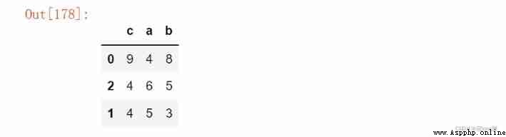
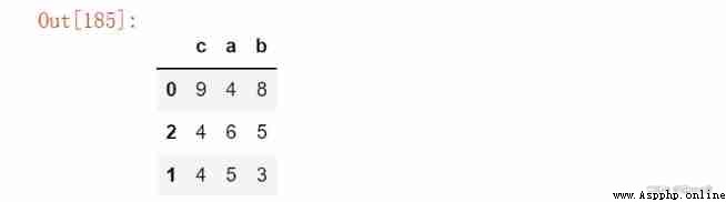
df = pd.DataFrame(arr, index = [0,2,1], columns = list('cab'))
# Alone DataFrame Sort a column of 
df.sort_values(by = ['c','a'], ascending = False)

3.3 Rank

Get the sorting of each element in the corresponding column from small to large . The common parameters are as follows ：

• method = ‘average’
  ‘average’： When the size is the same , Take the average value as the order
  ‘max’： When the size is the same , Take the maximum serial number
  ‘min’： When the size is the same , Take the minimum serial number
  ‘first’： When the size is the same , According to the storage order in memory

df.rank() # Get the ranking of each element in the corresponding column from small to large 
df.rank(method = 'first') # The default is average, first It means to sort by memory in the same order 
df.rank(method = 'min') # min max When it means the same, take min or max
df.rank(method = 'max') # min max When it means the same, take min or max

3.4 merge（ Match merge by column ）

• pd.merge(df1, df2, on = ‘X’, how = ‘inner’)
  take df1, df2 according to X Property merge . The possible ways are inner_join（ Only matching items ）, left_join（df2 Yes df1 Describe ）, right_join（df1 Yes df2 Describe ）, outer_join（ Include all items , If there is no match, it is NaN）.
  inner Output only matching items ,left, right Output the specified item ,outer Output all items .

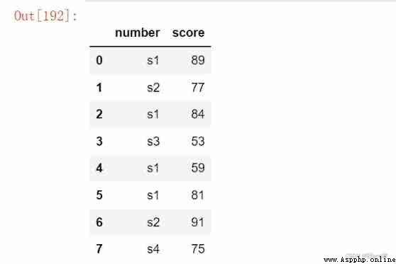
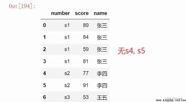
df1 = pd.DataFrame({

'number': ['s1', 's2', 's1', 's3', 's1', 's1', 's2', 's4'],
'score': np.random.randint(50, 100, size = 8),
})
df1
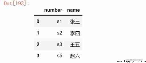
df2 = pd.DataFrame({

'number': ['s1', 's2', 's3', 's5'],
'name': [' Zhang San ', ' Li Si ', ' Wang Wu ', ' Zhao Liu ']
})
df2

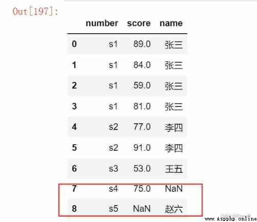
pd.merge(df1, df2, on = 'number') # inner_join How to connect 

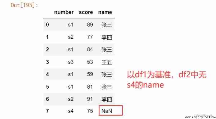
pd.merge(df1, df2, on = 'number', how = 'left') # Left connection 

pd.merge(df1, df2, on = 'number', how = 'right') # The right connection 

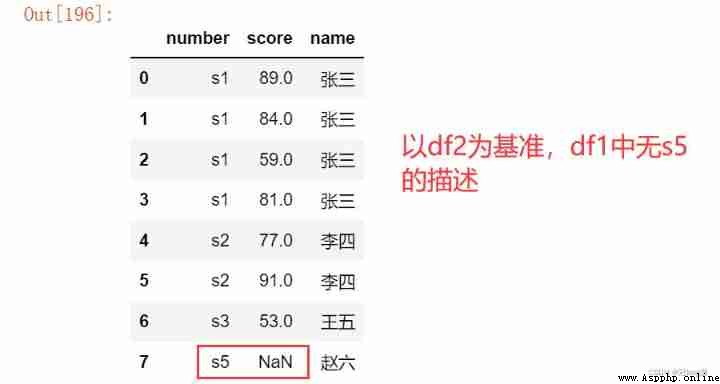
pd.merge(df1, df2, on = 'number', how = 'outer') # The right connection 

3.5 concat（ Data splicing ）

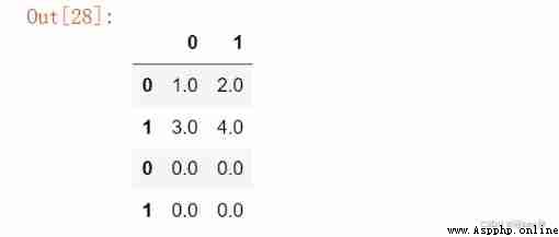
When we have multiple tables that need to be spliced together , May adopt concat Perform table splicing

• concat([df1, df2], axis = 0)
  take df1, df2 The longitudinal （axis = 0 Default ） Or horizontally （axis = 1） Splicing

data = np.arange(1, 5).reshape(2,-1)
df1 = pd.DataFrame(data)
df2 = pd.DataFrame(np.zeros((2,2)))
# Data splicing 
pd.concat([df1, df2])
# Data splicing 
pd.concat([df1, df2], axis = 1)

4. Data summary

1. describe
2. info
3. count
4. mean
5. sum

Data processing steps

1. Data analysis ： adopt head(5), tail(5) View the first and last elements , Understand the data structure .
2. Special value view ： adopt info(), describe() View includes NaN、 Element number 、 Standard deviation 、 Median and other special values

4.1 Special values （info, describe）

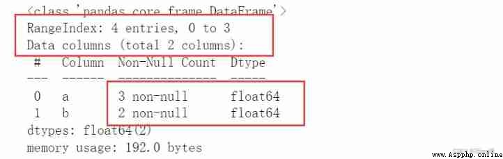
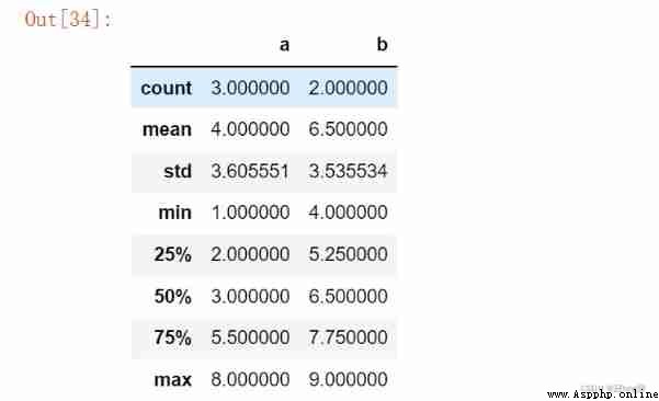
data = [
[1, None],
[None, None],
[8, 9],
[3, 4]
]
df = pd.DataFrame(data, columns = ['a', 'b'])
# The first step in data processing ： data structure + Special values head() -> info() --> describe()
df.info() # The ranks of 、 data type 、None Number of values and column distribution 、 Memory footprint 
df.describe() # The number of data 、 Distribution description 

4.2 Grouping statistics

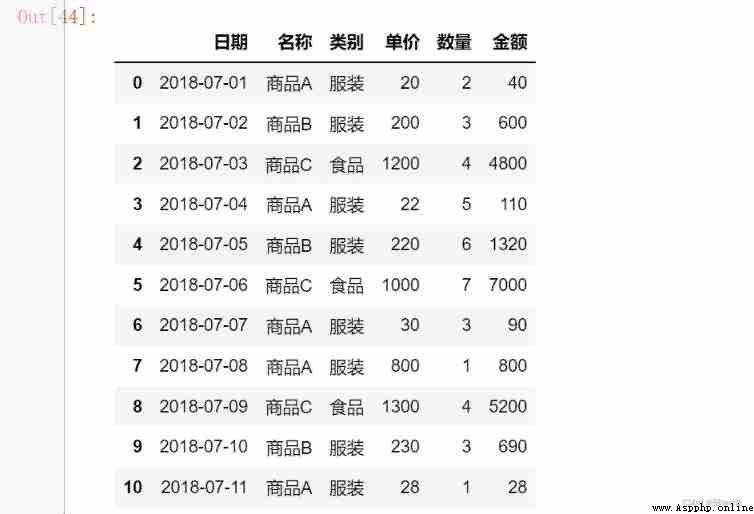
DataFrame Available through groupby(‘X’) function , With X or [X,…] Don't leave DataFrame division . Through the use of different classification levels, such as sum(), max() Such as function , Count the number of each category . You can also use for loop , Output classification results .

import xlrd
df = pd.read_excel('D:\\Jupyter_notebook\\pandas_data\\data.xlsx')
df

# Classified statistics 
grouped = df.groupby(' Category ')
for name, data in grouped:
print(name)
print(data)
# Elements of each category 
for name, data in grouped:
print(name)
print(data[' name '].unique())

clothing
date name Category The unit price Number amount of money
0 2018-07-01 goods A clothing 20 2 40
1 2018-07-02 goods B clothing 200 3 600
3 2018-07-04 goods A clothing 22 5 110
4 2018-07-05 goods B clothing 220 6 1320
6 2018-07-07 goods A clothing 30 3 90
7 2018-07-08 goods A clothing 800 1 800
9 2018-07-10 goods B clothing 230 3 690
10 2018-07-11 goods A clothing 28 1 28
food
date name Category The unit price Number amount of money
2 2018-07-03 goods C food 1200 4 4800
5 2018-07-06 goods C food 1000 7 7000
8 2018-07-09 goods C food 1300 4 5200

---

clothing
[‘ goods A’ ‘ goods B’]
food
[‘ goods C’]

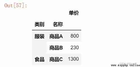
grouped = df.groupby([' Category ', ' name '])
grouped[[' The unit price ']].max()

5. The time series

1. datetime
2. time
3. date_range：date_range(start, end, freq= , periods=) Generating time series
4. to_datetime： take date_range() The generated time series are converted into time indexes
5. set_index
6. resample： Resampling , Reorganize the sampling frequency of the time series

5.1 Initialize time series

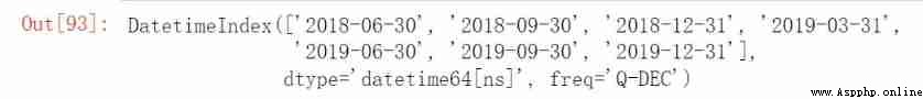
Pandas Use pd.date_range() Initialize time series . There are two initialization methods .

• Specify the start and end time
• Specify the start time and required number

among date_range() Contains two important parameters ：

1. freq = ‘D’： Set the sequence frequency . The default is D One day is the unit , There are common ‘w’： Zhou ,‘M’： month ,‘Q’： quarter ,‘H’： when ,‘T’： branch ,‘S’： second
2. period： Specify the number of sequences

pd.date_range('2018-5-1', '2020-2-15',freq = 'Q')
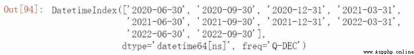
# Unknown start date , Appoint periods length 
pd.date_range('2020-05-01', freq = 'Q', periods = 10)

5.2 Time index

from date_range The generated time series cannot be directly used as a time index . need ==to_datetime()== Function to convert it to an index .
After converting time to index , The convenience of time reference will be greatly improved .

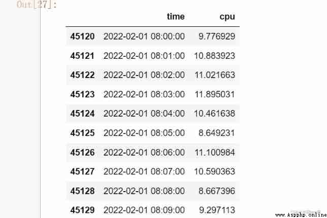
from datetime import datetime
import numpy as np
data = {

'time': pd.date_range('2022-01-01', periods = 200000, freq = 'T'),
'cpu' : np.random.randn(200000) + 10
}
df = pd.DataFrame(data)
df
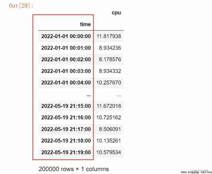
# Let time be the index 
s = pd.to_datetime(df.time)
df.index = s
df = df.drop('time', axis = 1)
df

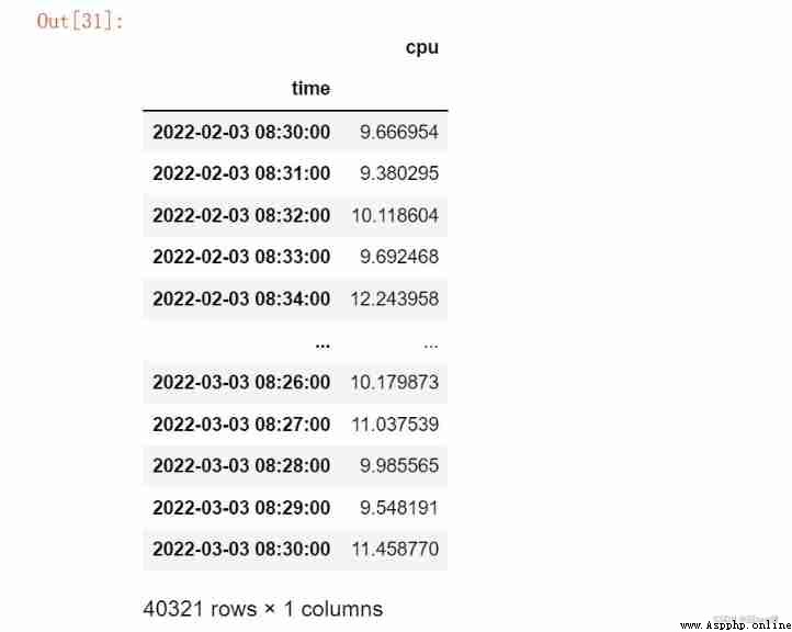
A certain period of time

df['2022-02-03 08:30:00':'2022-03-03 08:30:00']

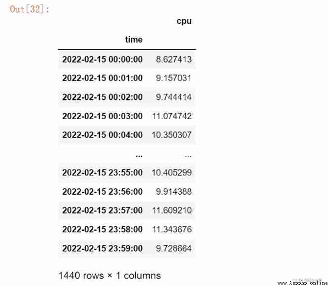
Specify time

df['2022-02-15']

grouping

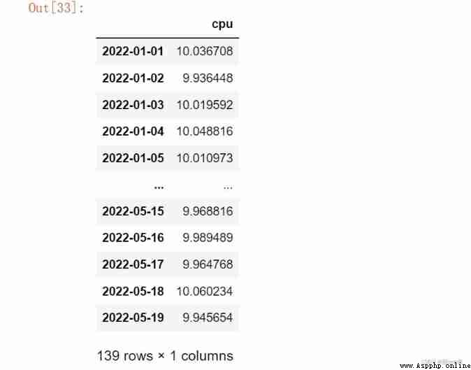
df.groupby(df.index.date).mean() # date Day grouping 

5.3 Resampling

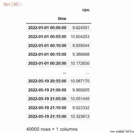
adopt resample() Function to resample a time series , Common parameters ：

• ‘nT’： Said to n Resample at a frequency of minutes . Common ones are ’H’, ‘S’, ‘Q’, ‘W’, ‘D’

# Resampling 
df.resample('5T').mean()

Reference material

[1] https://edu.csdn.net/learn/26273/326984