您现在的位置：程式師世界 >> 編程語言 > >> 更多編程語言 >> Python

Learning Python for beginners, self built 6-layer neural network, training fashion MNIST dataset -- the first door

編輯：Python

A general example of an introduction to deep learning is MNIST Training and testing , Almost even in the field of deep learning HELLO WORLD 了 , however , There is a problem ,MNIST Too simple. , Beginners construct casually with their glasses closed Several layers of network The accuracy can be improved to 90% above . however , Is this a beginner ？

The answer is no .

Examples of real-world development are not so simple , If you let beginners go straight to it VOC Or is it COCO Such data sets , It is possible that the accuracy of the neural network built by ourselves is not more than 30%.

Yes , If we don't use open source VGG、GooLeNet、ResNet wait , Maybe the hit rate of your code is not high .

This article introduces how to use Pytorch Train a self built neural network To train Fashion-MNIST Data sets .

Fashion-MNIST

Fashion-MINST The aim is to replace MNIST.

This is its address ：https://github.com/zalandoresearch/fashion-mnist

It's a collection of clothing pictures , All in all 10 Categories .

60000 Training pictures ,10000 Test pictures .

LabelDescription0T-shirt/top1Trouser2Pullover3Dress4Coat5Sandal6Shirt7Sneaker8Bag9Ankle boo

Fashion-MNIST It's not big , More convenient is like Tensorflow and Pytorch The current version can be downloaded directly with code .

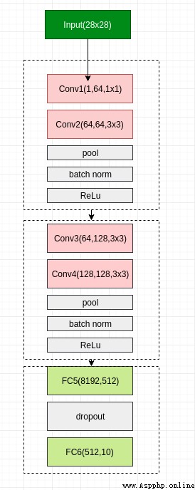
The steps of training neural networks

The following picture is made by myself , Every time I have to blog about it , I'll go over it and review it .

It reminds me to do these things ：

Processing data
Build a model
determine Loss function
Training

The following article will follow such steps to explain

Processing data

Download data

Pytorch Now through ready-made API You can download Fashion-MINST The data of

trainset = torchvision.datasets.FashionMNIST(root='./data', train=True, download=True, transform=transform)
trainloader = torch.utils.data.DataLoader(trainset, batch_size=100, shuffle=True, num_workers=2)
testset = torchvision.datasets.FashionMNIST(root='./data', train=False, download=True, transform=transform1)
testloader = torch.utils.data.DataLoader(testset, batch_size=50, shuffle=False, num_workers=2)

It creates two DataLoader , Separately used for load Pictures of training set and test set .

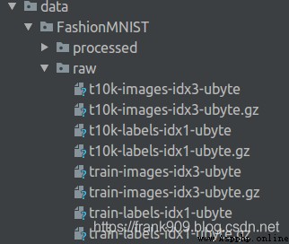
After the code runs , Will be in Current directory data Catalog Save the corresponding file in the .

Data to enhance

In order to improve the generalization Ability , Generally, the data will be enhance operation .

transform = transforms.Compose(
[
transforms.RandomHorizontalFlip(),
transforms.RandomGrayscale(),
transforms.ToTensor()])
transform1 = transforms.Compose(
[
transforms.ToTensor()])

transform It's mainly about turning left and right , Gray level random transformation , Used to enhance the training image , The test picture is not needed .

transform The reference to the previous dataset is passed to the corresponding API That's all right. , Very convenient .

Build a model

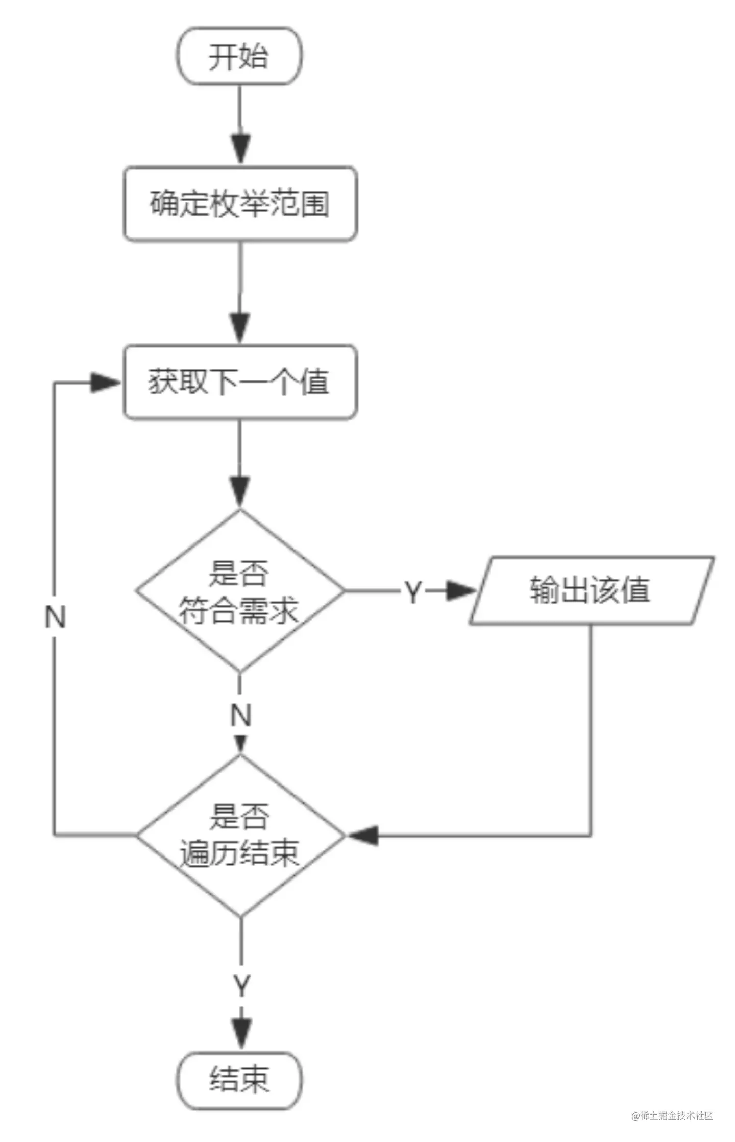
Although it's a neural network built by ourselves , But it refers to VGG The network architecture of .

in total 6 Layer of the network ,4 Convolution layer ,2 Layer full connection .

use Pytorch It's also very convenient to implement .

class Net(nn.Module):
def __init__(self):
super(Net,self).__init__()
self.conv1 = nn.Conv2d(1,64,1,padding=1)
self.conv2 = nn.Conv2d(64,64,3,padding=1)
self.pool1 = nn.MaxPool2d(2, 2)
self.bn1 = nn.BatchNorm2d(64)
self.relu1 = nn.ReLU()
self.conv3 = nn.Conv2d(64,128,3,padding=1)
self.conv4 = nn.Conv2d(128, 128, 3,padding=1)
self.pool2 = nn.MaxPool2d(2, 2, padding=1)
self.bn2 = nn.BatchNorm2d(128)
self.relu2 = nn.ReLU()
self.fc5 = nn.Linear(128*8*8,512)
self.drop1 = nn.Dropout2d()
self.fc6 = nn.Linear(512,10)
def forward(self,x):
x = self.conv1(x) # Convolution 
x = self.conv2(x)
x = self.pool1(x) # The Internet 1
x = self.bn1(x) # The Internet 2
x = self.relu1(x) # The Internet 3
x = self.conv3(x)
x = self.conv4(x)
x = self.pool2(x) # The Internet 4
x = self.bn2(x) # The Internet 5
x = self.relu2(x) # The Internet 6
#print(" x shape ",x.size())
x = x.view(-1,128*8*8)
x = F.relu(self.fc5(x)) # Full connection 1
x = self.drop1(x)
x = self.fc6(x) # Full connection 2
return x

It is worth noting that , After the convolution layer, I used Batch Norm The means of , In the full connectivity layer, I used Dropout, Both aim to reduce Over fitting The phenomenon of .

Develop training strategies

I chose the more popular Adam As optimization section , Learning rate yes 0.0001.

then ,loss choose Cross entropy .

 def train_sgd(self,device,epochs=100):
optimizer = optim.Adam(self.parameters(), lr=0.0001)
path = 'weights.tar'
initepoch = 0
if os.path.exists(path) is not True:
loss = nn.CrossEntropyLoss()
# optimizer = optim.SGD(self.parameters(),lr=0.01)
else:
checkpoint = torch.load(path)
self.load_state_dict(checkpoint['model_state_dict'])
optimizer.load_state_dict(checkpoint['optimizer_state_dict'])
initepoch = checkpoint['epoch']
loss = checkpoint['loss']
for epoch in range(initepoch,epochs): # loop over the dataset multiple times
timestart = time.time()
running_loss = 0.0
total = 0
correct = 0
for i, data in enumerate(trainloader, 0):
# get the inputs
inputs, labels = data
inputs, labels = inputs.to(device),labels.to(device)
# zero the parameter gradients
optimizer.zero_grad()
# forward + backward + optimize
outputs = self(inputs)
l = loss(outputs, labels)
l.backward()
optimizer.step()
# print statistics
running_loss += l.item()
# print("i ",i)
if i % 500 == 499: # print every 500 mini-batches
print('[%d, %5d] loss: %.4f' %
(epoch, i, running_loss / 500))
running_loss = 0.0
_, predicted = torch.max(outputs.data, 1)
total += labels.size(0)
correct += (predicted == labels).sum().item()
print('Accuracy of the network on the %d tran images: %.3f %%' % (total,
100.0 * correct / total))
total = 0
correct = 0
torch.save({
'epoch':epoch,
'model_state_dict':net.state_dict(),
'optimizer_state_dict':optimizer.state_dict(),
'loss':loss
},path)
print('epoch %d cost %3f sec' %(epoch,time.time()-timestart))
print('Finished Training')

The above code also has the function of saving and loading models .

adopt save()
Can save network training state .

torch.save({
'epoch':epoch,
'model_state_dict':net.state_dict(),
'optimizer_state_dict':optimizer.state_dict(),
'loss':loss
},path)

I defined... In the code path by weights.tar, When the task is executed , The model data will also be saved .
adopt load()
Can load saved model data .

checkpoint = torch.load(path)
self.load_state_dict(checkpoint['model_state_dict'])
optimizer.load_state_dict(checkpoint['optimizer_state_dict'])
initepoch = checkpoint['epoch']
loss = checkpoint['loss']

test

Testing is a little different from training , It just needs forward derivation .

 def test(self,device):
correct = 0
total = 0
with torch.no_grad():
for data in testloader:
images, labels = data
images, labels = images.to(device), labels.to(device)
outputs = self(images)
_, predicted = torch.max(outputs.data, 1)
total += labels.size(0)
correct += (predicted == labels).sum().item()
print('Accuracy of the network on the 10000 test images: %.3f %%' % (
100.0 * correct / total))

Training results

The following code for training and verification .

if __name__ == "__main__":
device = torch.device("cuda:0" if torch.cuda.is_available() else "cpu")
net = Net()
net = net.to(device)
net.train_sgd(device,30)
net.test(device)

The code will depend on whether the machine has cuda equipment To decide what training to use , For example, the machine is not installed GPU, Then it will use CPU perform , It's going to be a little bit slower .

Because the model is simple , I chose training 30 individual epoch On termination .

Last , You can run the code .

my Pytorch The version is 1.2,Cuda The version is 10.1,GPU yes 1080 Ti.

Run one epoch It will probably take 6 A second more .

after 30 individual epoch after , The training accuracy can reach 99%, The test accuracy can be 92.29%.

[0, 499] loss: 0.4572
Accuracy of the network on the 100 tran images: 87.000 %
epoch 0 cost 7.158301 sec
[1, 499] loss: 0.2840
Accuracy of the network on the 100 tran images: 90.000 %
epoch 1 cost 6.451613 sec
[2, 499] loss: 0.2458
Accuracy of the network on the 100 tran images: 95.000 %
epoch 2 cost 6.450977 sec
[3, 499] loss: 0.2197
Accuracy of the network on the 100 tran images: 92.000 %
epoch 3 cost 6.383819 sec
[4, 499] loss: 0.2009
Accuracy of the network on the 100 tran images: 90.000 %
epoch 4 cost 6.443048 sec
[5, 499] loss: 0.1840
Accuracy of the network on the 100 tran images: 94.000 %
epoch 5 cost 6.411542 sec
[6, 499] loss: 0.1688
Accuracy of the network on the 100 tran images: 94.000 %
epoch 6 cost 6.420368 sec
[7, 499] loss: 0.1584
Accuracy of the network on the 100 tran images: 93.000 %
epoch 7 cost 6.390420 sec
[8, 499] loss: 0.1452
Accuracy of the network on the 100 tran images: 93.000 %
epoch 8 cost 6.473319 sec
[9, 499] loss: 0.1342
Accuracy of the network on the 100 tran images: 96.000 %
epoch 9 cost 6.435586 sec
[10, 499] loss: 0.1275
Accuracy of the network on the 100 tran images: 95.000 %
epoch 10 cost 6.422722 sec
[11, 499] loss: 0.1177
Accuracy of the network on the 100 tran images: 96.000 %
epoch 11 cost 6.490834 sec
[12, 499] loss: 0.1085
Accuracy of the network on the 100 tran images: 96.000 %
epoch 12 cost 6.499629 sec
[13, 499] loss: 0.1021
Accuracy of the network on the 100 tran images: 92.000 %
epoch 13 cost 6.512994 sec
[14, 499] loss: 0.0929
Accuracy of the network on the 100 tran images: 96.000 %
epoch 14 cost 6.510045 sec
[15, 499] loss: 0.0871
Accuracy of the network on the 100 tran images: 94.000 %
epoch 15 cost 6.422577 sec
[16, 499] loss: 0.0824
Accuracy of the network on the 100 tran images: 98.000 %
epoch 16 cost 6.577342 sec
[17, 499] loss: 0.0749
Accuracy of the network on the 100 tran images: 97.000 %
epoch 17 cost 6.491562 sec
[18, 499] loss: 0.0702
Accuracy of the network on the 100 tran images: 99.000 %
epoch 18 cost 6.430238 sec
[19, 499] loss: 0.0634
Accuracy of the network on the 100 tran images: 98.000 %
epoch 19 cost 6.540339 sec
[20, 499] loss: 0.0631
Accuracy of the network on the 100 tran images: 97.000 %
epoch 20 cost 6.490717 sec
[21, 499] loss: 0.0545
Accuracy of the network on the 100 tran images: 98.000 %
epoch 21 cost 6.583902 sec
[22, 499] loss: 0.0535
Accuracy of the network on the 100 tran images: 98.000 %
epoch 22 cost 6.423389 sec
[23, 499] loss: 0.0491
Accuracy of the network on the 100 tran images: 99.000 %
epoch 23 cost 6.573753 sec
[24, 499] loss: 0.0474
Accuracy of the network on the 100 tran images: 95.000 %
epoch 24 cost 6.577250 sec
[25, 499] loss: 0.0422
Accuracy of the network on the 100 tran images: 98.000 %
epoch 25 cost 6.587380 sec
[26, 499] loss: 0.0416
Accuracy of the network on the 100 tran images: 98.000 %
epoch 26 cost 6.595343 sec
[27, 499] loss: 0.0402
Accuracy of the network on the 100 tran images: 99.000 %
epoch 27 cost 6.748190 sec
[28, 499] loss: 0.0366
Accuracy of the network on the 100 tran images: 99.000 %
epoch 28 cost 6.554550 sec
[29, 499] loss: 0.0327
Accuracy of the network on the 100 tran images: 97.000 %
epoch 29 cost 6.475854 sec
Finished Training
Accuracy of the network on the 10000 test images: 92.290 %

92% What's the level ？ Given earlier Fashion-MNIST The address given can be in benchmark Top of the list .

Website display Fashion-MNIST The highest score on the test is 96.7%, It shows that my model can be optimized and worked hard .

The follow-up to optimize

Because I built the model at random , It's just absorbing more advanced means , More layers can be tried on this basis , Fewer parameters .
Patient adjustment of parameters , The study rate is what I give casually , Whether it is reasonable is not verified .
ResNet When doing image recognition , More powerful , We can try to introduce Residual unit .
visualization , Maybe a lot of novices are not good at it , What's your training stuff , So you can try to show some intermediate results yourself .
Complete code ：

import torch
import torch.nn as nn
import torch.nn.functional as F
import torchvision
import torchvision.transforms as transforms
import torch.optim as optim
import time
import os
transform = transforms.Compose(
[
transforms.RandomHorizontalFlip(),
transforms.RandomGrayscale(),
transforms.ToTensor()])
transform1 = transforms.Compose(
[
transforms.ToTensor()])
trainset = torchvision.datasets.FashionMNIST(root='./data', train=True,
download=True, transform=transform)
trainloader = torch.utils.data.DataLoader(trainset, batch_size=100,
shuffle=True, num_workers=2)
testset = torchvision.datasets.FashionMNIST(root='./data', train=False,
download=True, transform=transform1)
testloader = torch.utils.data.DataLoader(testset, batch_size=50,
shuffle=False, num_workers=2)
classes = ('T-shirt', 'Trouser', 'Pullover', 'Dress',
'Coat', 'Sandal', 'Shirt', 'Sneaker', 'Bag', 'Ankle boot')
class Net(nn.Module):
def __init__(self):
super(Net,self).__init__()
self.conv1 = nn.Conv2d(1,64,1,padding=1)
self.conv2 = nn.Conv2d(64,64,3,padding=1)
self.pool1 = nn.MaxPool2d(2, 2)
self.bn1 = nn.BatchNorm2d(64)
self.relu1 = nn.ReLU()
self.conv3 = nn.Conv2d(64,128,3,padding=1)
self.conv4 = nn.Conv2d(128, 128, 3,padding=1)
self.pool2 = nn.MaxPool2d(2, 2, padding=1)
self.bn2 = nn.BatchNorm2d(128)
self.relu2 = nn.ReLU()
self.fc5 = nn.Linear(128*8*8,512)
self.drop1 = nn.Dropout2d()
self.fc6 = nn.Linear(512,10)
def forward(self,x):
x = self.conv1(x)
x = self.conv2(x)
x = self.pool1(x)
x = self.bn1(x)
x = self.relu1(x)
x = self.conv3(x)
x = self.conv4(x)
x = self.pool2(x)
x = self.bn2(x)
x = self.relu2(x)
#print(" x shape ",x.size())
x = x.view(-1,128*8*8)
x = F.relu(self.fc5(x))
x = self.drop1(x)
x = self.fc6(x)
return x
def train_sgd(self,device,epochs=100):
optimizer = optim.Adam(self.parameters(), lr=0.0001)
path = 'weights.tar'
initepoch = 0
if os.path.exists(path) is not True:
loss = nn.CrossEntropyLoss()
# optimizer = optim.SGD(self.parameters(),lr=0.01)
else:
checkpoint = torch.load(path)
self.load_state_dict(checkpoint['model_state_dict'])
optimizer.load_state_dict(checkpoint['optimizer_state_dict'])
initepoch = checkpoint['epoch']
loss = checkpoint['loss']
for epoch in range(initepoch,epochs): # loop over the dataset multiple times
timestart = time.time()
running_loss = 0.0
total = 0
correct = 0
for i, data in enumerate(trainloader, 0):
# get the inputs
inputs, labels = data
inputs, labels = inputs.to(device),labels.to(device)
# zero the parameter gradients
optimizer.zero_grad()
# forward + backward + optimize
outputs = self(inputs)
l = loss(outputs, labels)
l.backward()
optimizer.step()
# print statistics
running_loss += l.item()
# print("i ",i)
if i % 500 == 499: # print every 500 mini-batches
print('[%d, %5d] loss: %.4f' %
(epoch, i, running_loss / 500))
running_loss = 0.0
_, predicted = torch.max(outputs.data, 1)
total += labels.size(0)
correct += (predicted == labels).sum().item()
print('Accuracy of the network on the %d tran images: %.3f %%' % (total,
100.0 * correct / total))
total = 0
correct = 0
torch.save({
'epoch':epoch,
'model_state_dict':net.state_dict(),
'optimizer_state_dict':optimizer.state_dict(),
'loss':loss
},path)
print('epoch %d cost %3f sec' %(epoch,time.time()-timestart))
print('Finished Training')
def test(self,device):
correct = 0
total = 0
with torch.no_grad():
for data in testloader:
images, labels = data
images, labels = images.to(device), labels.to(device)
outputs = self(images)
_, predicted = torch.max(outputs.data, 1)
total += labels.size(0)
correct += (predicted == labels).sum().item()
print('Accuracy of the network on the 10000 test images: %.3f %%' % (
100.0 * correct / total))
if __name__ == "__main__":
device = torch.device("cuda:0" if torch.cuda.is_available() else "cpu")
net = Net()
net = net.to(device)
net.train_sgd(device,30)
net.test(device)