Hello everyone , I'm Junxin
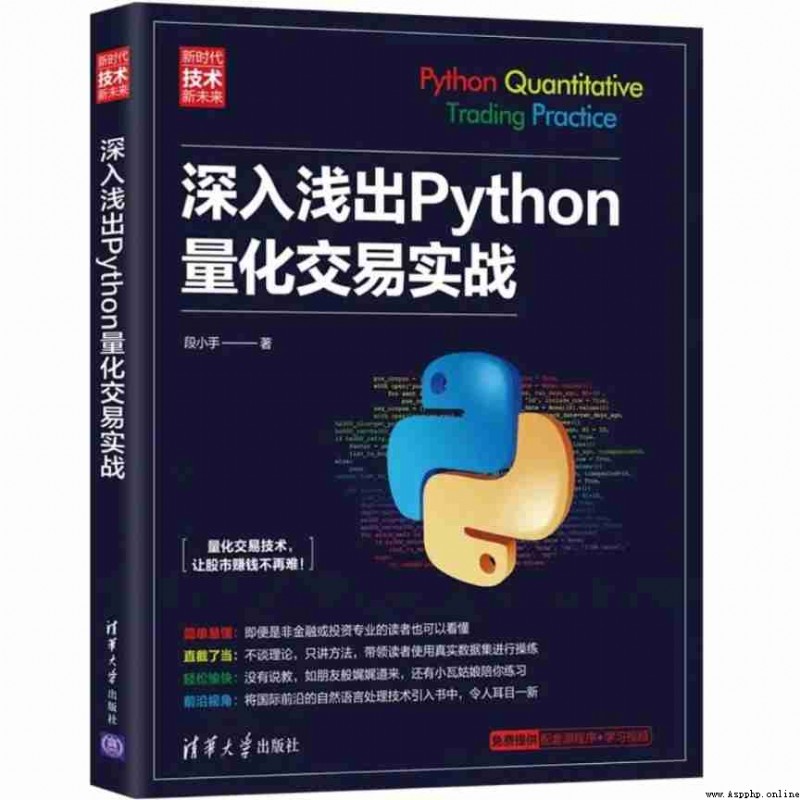
Not long ago , Received a gift from Tsinghua University Press 《 Explain profound theories in simple language Python Quantitative trading practice 》 A Book , Also promised the publishing house Write some reading notes , I'll hand in my homework today .
Of course the old rule , Junxin will be in this chapter Total gifts 3 This book , See the rules at the end of the text .
Here are some simple attempts I made with reference to the contents of the book , For reference only . This book is for the use of Python Beginners who play quantification , It's still friendly , If you are interested, you can consider starting a book .
use Python Plot the price of the stock 5 The daily average and 20 ma . as everyone knows ,5 The daily average is the life and death line of short-term trading , and 20 The daily moving average is the watershed of the medium and long-term trend . therefore , Based on these two moving averages , You can design some simple trading strategies .
Here is the code I practiced :
import pandas as pd
import numpy as np
from pandas_datareader import data
import datetime
import matplotlib.pyplot as plt
Import part of the library , No explanation. , Pull data below :
end_date = datetime.date.today()
start_date = end_date - datetime.timedelta(days = 100)
price = data.DataReader('601127.ss','yahoo',
start_date,
end_date)
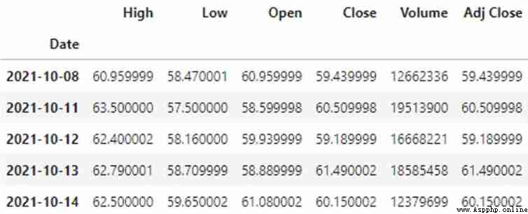
price.head()Here I choose from yahoo PULL 601127 This stock used to 100 Days of market data . Can see the earliest data to 2021 Year of 10 month 8 Japan :
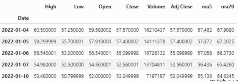
Then I started adding 5 Day and 20 ma
price['ma5'] = price['Adj Close'].rolling(5).mean()
price['ma20'] = price['Adj Close'].rolling(20).mean()
price.tail()
You can see in the data :
For the convenience of observation , I drew a picture with code :
fig = plt.figure(figsize=(16,9))
ax1 = fig.add_subplot(111, ylabel='Price')
price['Adj Close'].plot(ax=ax1, color='g', lw=2., legend=True)
price.ma5.plot(ax=ax1, color='r', lw=2., legend=True)
price.ma20.plot(ax=ax1, color='b', lw=2., legend=True)
plt.grid()
plt.show()
So you can see the image directly :
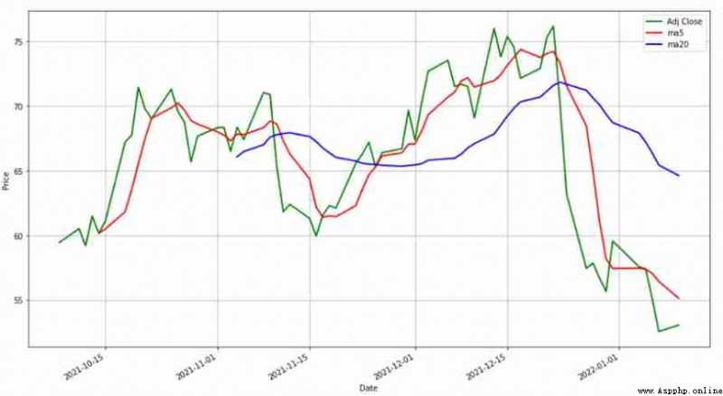
In this way, we can design the moving average strategy according to the moving average of different periods .
Here we use the words in the book KNN Trading strategy of mode , Replaced by a logistic regression model , Try to see how the performance of the strategy will change .
Without saying , Go up the ladder , Guide Kula data :
import pandas as pd
import pandas_datareader.data as web
import numpy as np
from datetime import datetime
There's not much data , To a 3 Year of :
end = datetime.date.today()
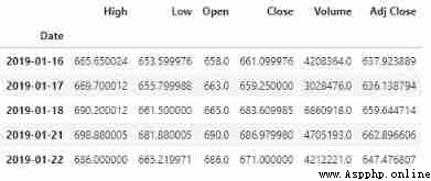
start = end - datetime.timedelta(days = 365*3)I'm big A stocks , Best cattle X Shares , To say Maotai , No one is against it ? Let's do the market data of Maotai :
owB = web.DataReader('600519.ss', 'yahoo',
                     start,
                     end)
cowB.head()
When he pulled it down, Ben Xian was surprised ,2019 year 1 In the month , Da Maotai CAI 600 How much money ! However, it is estimated that benxian was asked to buy , Ben Xian dare not . At that time, I was old A There are not many stocks with more than 100 shares !
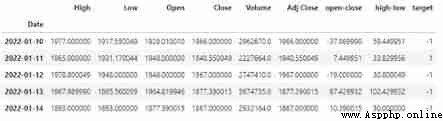
Then I follow the method in the book , Do feature Engineering :
cowB['open-close'] = cowB['Open'] - cowB ['Close']
cowB ['high-low'] = cowB ['High'] - cowB ['Low']
cowB ['target'] = np.where(cowB ['Close'].shift(-1) > cowB ['Close'],1,-1)
cowB = cowB.dropna()
cowB.tail()
Then there are a few more columns ,target Inside ,1 It means rising the next day ,-1 It means falling the next day :
Now we're going to make a model :
x = cowB [['open-close','high-low']]
y = cowB ['target']
Split into x and y, Then please go out scikit-learn:
from sklearn.model_selection import train_test_split
from sklearn.linear_model import LogisticRegression
Then the data set is divided into training set and test set :
x_train, x_test, y_train, y_test =\
train_test_split(x, y, train_size = 0.8)
See how logistic regression performs :
lr = LogisticRegression()
lr.fit(x_train, y_train)
print(lr.score(x_train, y_train))
print(lr.score(x_test, y_test))
Results found , Not in the book yet KNN The score is high :
0.5438898450946644
0.5136986301369864
The accuracy of logistic regression in the training set is 54.39%, And in the book KNN The accuracy rate is basically the same ; But there are only 51.37%, Than in the book KNN The model is almost lower 3 percentage .
The result of the second note is a little heartbreaking , But the goal is to try , Spare time to play , If you are interested, you can also practice by yourself .
Book donation
Give away books cadastral :3 Ben 《 Explain profound theories in simple language Python Quantitative trading practice 》, from 「 tsinghua university press 」 Sponsorship provides ,Python Quantitative classics , It is strongly recommended to start a book .
Gift rules : Send it out by leaving a message and liking ,「 Forward this article to the circle of friends 」+「 Leaving a message. 」, The number of comments and likes is the largest front 3 position The reader will receive a ( Only when you leave a message can you select ). Opening time :「2 month 25 Japan 20:00」.
matters needing attention : The final recipient is requested to 24 Add my wechat within hours :1072362067, remarks : present sb. with a book , And provide screenshots of circle of friends forwarding and collecting likes . If the machine or non real traffic is found, brush like , After discovery, it will be blacklisted , Disqualification .